Axicon¶

class raytracing.Axicon(alpha, n, diameter=inf, label='')¶

Bases: raytracing.matrix.Matrix

This class is an advanced module that describes an axicon lens, not part of the basic formalism. Using this class an axicon conical lens can be presented. Axicon lenses are used to obtain a line focus instead of a point. The formalism is described in Kloos, sec. 2.2.3

Parameters:

alpha (float) – alpha is the small angle in radians of the axicon (typically 2.5 or 5 degrees) corresponding to 90-apex angle
n (float) – index of refraction. This value cannot be less than 1.0. It is assumed the axicon is in air.
diameter (float) – Aperture of the element. (default = +Inf) The diameter of the aperture must be a positive value.
label (string) – The label of the axicon lens.

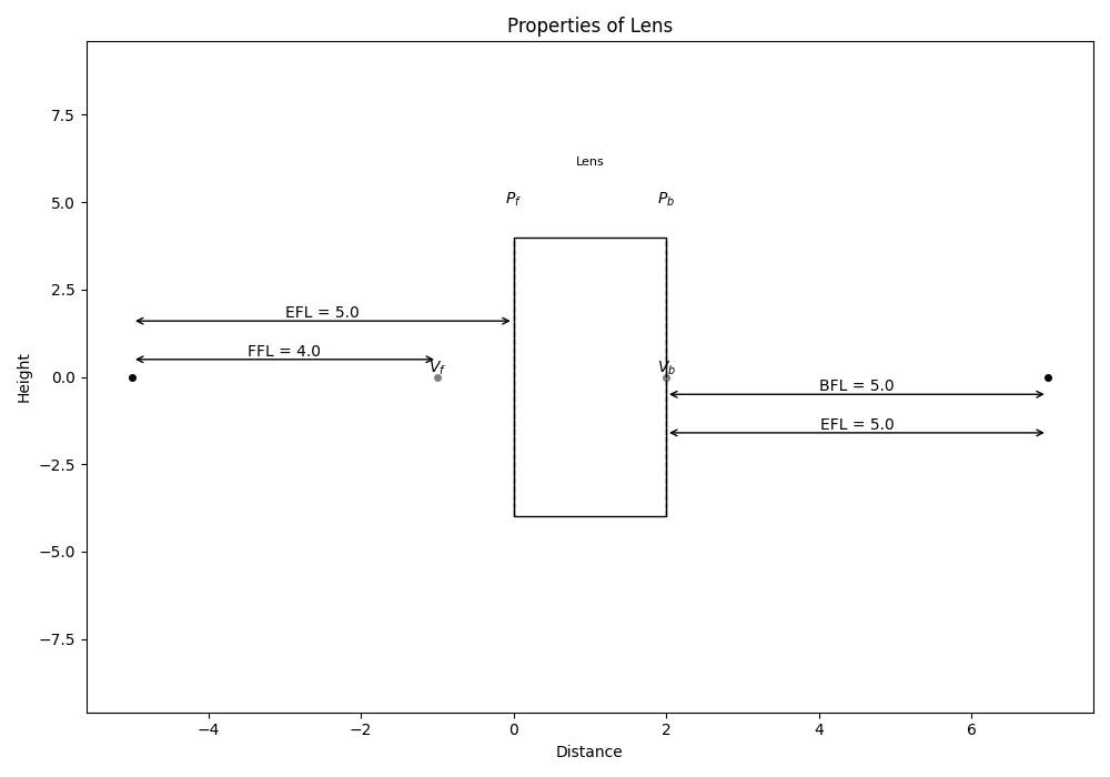
backFocalLength()¶

The focal lengths measured from the back vertex. This is the distance between the surface and the focal point. When the principal plane is not at the surface (which is usually the case in anything except a thin lens), the back and front focal lengths will be different from effective focal lengths. The effective focal lengths is always measured from the principal planes, but the BFL and FFL are measured from the vertex.

Returns:	backFocalLength – Returns the BFL
Return type:	float

Examples

Since this function returns the BFL, if the focal distance of an object is 5 and the back vertex is 2, we expect to have back focal length of 3, as the following example:

>>> from raytracing import *
>>> # M1 is an ABCD matrix of a lens (f=5)
>>> M1= Matrix(A=1,B=0,C=-1/5,D=1,physicalLength=0,backVertex=2,label='Lens')
>>> BFL=M1.backFocalLength()
>>> print('the back focal distance:' , BFL)
the back focal distance: 3.0

Notes

If the matrix is the result of the product of several matrices, we may not know where the front and back vertices are. In that case, we return None (or undefined).

The front and back focal lengths will be different if the index of refraction is different on both sides.

backwardConjugate()¶

With an image at the back edge of the element, where is the object ? Distance before the element by which a ray must travel to reach the conjugate plane at the back of the element. A positive distance means the object is “distance” in front of the element (or to the left, or before).

Returns:	backwardConjugate – index [0] output object is the distance of the image in front of the element and index [1] is the conjugate matrix.
Return type:	object

Examples

>>> from raytracing import *
>>> # M1 is an ABCD matrix of an object
>>> M1= Matrix(A=2,B=1,C=5,D=3,physicalLength=2,label='Lens')
>>> Image=M1.backwardConjugate()
>>> print('The position of the image:' , Image[0])
The position of the image: -0.5

>>> print(Image[1]) #print the conjugate matrix
|  2.000    0.000 |
|                 |
|  5.000    0.500 |
f=-0.200

See also

raytracing.Matrix.forwardConjugate()

Notes

M2 = M1*Space(distance) M2.isImaging == True

determinant¶: The determinant of the ABCD matrix is always frontIndex/backIndex, which is often 1.0. We make a calculation exception when C == 0 and B is infinity: since B is never really infinity, but C can be precisely zero (especially in free space), then B*C is zero in that particular case.

deviationAngle()¶

This function provides deviation angle delta assuming that the axicon is in air and that the incidence is near normal, which is the usual way of using an axicon.

Returns:	delta – the deviation angle
Return type:	float

See also

https(): //ru.b-ok2.org/book/2482970/9062b7, p.48

displayHalfHeight()¶

A reasonable height for display purposes for an element, whether it is infinite or not. If the element is infinite, the half-height is currently set to ‘4’ or to the specified minimum half height. If not, it is the apertureDiameter/2. :param minSize: The minimum size to be considered as the aperture half height :type minSize: float

Returns:	halfHeight – The half height of the optical element
Return type:	float

effectiveFocalLengths()¶

The effective focal lengths calculated from the power (C) of the matrix.

There are in general two effective focal lengths: front effective and back effective focal lengths (not to be confused with back focal and front focal lengths which are measured from the physical interface). The easiest way to calculate this is to use f = -1/C for current matrix, then flipOrientation and f = -1/C

Returns:	effectiveFocalLengths – Returns the effective focal lengths in the forward and backward directions. When in air, both are equal.
Return type:	array

See also

raytracing.Matrix.focalDistances()

Examples

>>> from raytracing import *
>>> # M1 is an ABCD matrix of a lens (f=5)
>>> M1= Matrix(A=1,B=0,C=-1/5,D=1,physicalLength=0,label='Lens')
>>> f2=M1.effectiveFocalLengths()
>>> print('focal distances:' , f2)
focal distances: FocalLengths(f1=5.0, f2=5.0)

This function has the same out put as effectiveFocalLengths() >>> f1=M1.focalDistances() >>> print(‘focal distances:’ , f1) focal distances: FocalLengths(f1=5.0, f2=5.0)

flipOrientation()¶

We flip the element around (as in, we turn a lens around front-back). This is useful for real elements and for groups.

Returns:	Matrix – An element with the properties of the flipped original element
Return type:	object of Matrix class

Examples

>>> # Mat is an ABCD matrix of an object
>>> Mat= Matrix(A=1,B=0,C=-1/5,D=1,physicalLength=2,frontVertex=-1,backVertex=2,label='Lens')
>>> Mat.display()
>>> flippedMat=Mat.flipOrientation()
>>> flippedMat.display()

The original object:

The flipped object:

See also

raytracing.Matrix()

Notes

For individual objects, it does not do anything because they are the same either way. However, subclasses can override this function and act accordingly.

focalDistances()¶

This is the synonym of effectiveFocalLengths()

Returns:	focalDistances – Returns the effective focal lengths on either side.
Return type:	array

Examples

>>> from raytracing import *
>>> # M1 is an ABCD matrix of a lens (f=5)
>>> M1= Matrix(A=1,B=0,C=-1/5,D=1,physicalLength=0,label='Lens')
>>> f1=M1.focalDistances()
>>> print('focal distances:' , f1)
focal distances: FocalLengths(f1=5.0, f2=5.0)

This function has the same out put as effectiveFocalLengths()

>>> f2=M1.effectiveFocalLengths()
>>> print('focal distances:' , f2)
focal distances: FocalLengths(f1=5.0, f2=5.0)

focalLineLength(yMax=None)¶

Provides the line length, assuming a ray at height yMax

Parameters:	yMax (float) – the height of the ray (default=None) If no height is defined for the ray, then yMax would be set to the height of the axicon (apertureDiameter/2)
Returns:	focalLineLength – the length of the focal line
Return type:	float

See also

https(): //ru.b-ok2.org/book/2482970/9062b7, p.48

focusPositions(z)¶

Positions of both focal points on either side of the element.

The front and back focal spots will be different if the index of refraction is different on both sides.

Parameters:	z (float) – Position from where the positions are calculated
Returns:	focusPositions – An array of front focal position and the back focal position.
Return type:	array

Examples

>>> from raytracing import *
>>> # M1 is an ABCD matrix of a lens (f=5)
>>> M1= Matrix(A=1,B=0,C=-1/5,D=1,physicalLength=4,frontVertex=-1,backVertex=5,label='Lens')
>>> Position0=M1.focusPositions(z=0)
>>> print('focal positions (F,B):' , Position0)
focal positions (F,B): CardinalPoint(z1=-5.0, z2=9.0)

And if we move object 2 units:

>>> Position2=M1.focusPositions(z=2)
>>> print('focal positions (F,B):' , Position2)
focal positions (F,B): CardinalPoint(z1=-3.0, z2=11.0)

forwardConjugate()¶

With an object at the front edge of the element, where is the image? Distance after the element by which a ray must travel to reach the conjugate plane of the front of the element. A positive distance means the image is “distance” beyond the back of the element (or to the right, or after).

Returns:	forwardConjugate – index [0] output object is the distance of the image at the back of the element and index [1] is the conjugate matrix.
Return type:	object

Examples

>>> from raytracing import *
>>> # M1 is an ABCD matrix of an object
>>> M1= Matrix(A=3,B=1,C=5,D=2,physicalLength=0,label='Lens')
>>> Image=M1.forwardConjugate()
>>> print('The position of the image:' , Image[0])
The position of the image: -0.5

>>> print(Image[1]) #print the conjugate matrix
|  0.500    0.000 |
|                 |
|  5.000    2.000 |
f=-0.200

See also

raytracing.Matrix.backwardConjugate()

Notes

M2 = Space(distance)*M1 M2.isImaging == True

forwardSurfaces¶: A list of surfaces that represents the element for drawing purposes

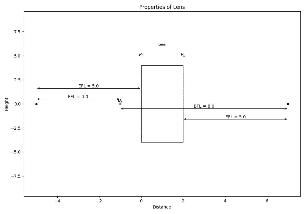
frontFocalLength()¶

The focal lengths measured from the front vertex. This is the distance between the surface and the focal point. When the principal plane is not at the surface (which is usually the case in anything except a thin lens), the back and front focal lengths will be different from effective focal lengths. The effective focal lengths is always measured from the principal planes, but the BFL and FFL are measured from the vertices.

Returns:	frontFocalLength – Returns the FFL
Return type:	float

Examples

In the following example, we have defined an object(f=5) with physical length of 4. And the front vertex is placed one unit before the front principal plane. There for the front focal length will be 4.

>>> from raytracing import *
>>> # M1 is an ABCD matrix of a lens (f=5)
>>> M1= Matrix(A=1,B=0,C=-1/5,D=1,physicalLength=4,frontVertex=-1,label='Lens')
>>> FFL=M1.frontFocalLength()
>>> print('the front focal distance:' , FFL)
the front focal distance: 4.0

Notes

If the matrix is the result of the product of several matrices, we may not know where the front and back vertices are. In that case, we return None (or undefined).

The front and back focal lengths will be different if the index of refraction is different on both sides.

hasFiniteApertureDiameter()¶

If the system has a finite aperture size

Returns:	apertureDiameter – If True, the element or group of elements have a finite aperture size
Return type:	bool

hasPower¶

If True, then there is a non-null focal length because C!=0. We compare to an epsilon value, because computational errors can occur and lead to C being very small, but not 0.

Examples

>>> from raytracing import *
>>> # M1 is an ABCD matrix of a lens (f=10)
>>> M1= Matrix(A=1,B=0,C=-1/10,D=1,physicalLength=2,label='Lens')
>>> print('hasPower:' , M1.hasPower)
hasPower: True

>>> # M2 is an ABCD matrix of free space (d=2)
>>> M2= Matrix(A=1,B=2,C=0,D=1,physicalLength=2,label='Lens')
>>> print('hasPower:' , M2.hasPower)
hasPower: False

isImaging¶

If B=0, then the matrix represents that transfer from a conjugate plane to another (i.e. object at the front edge and image at the back edge).

Examples

>>> from raytracing import *
>>> # M1 is an ABCD matrix of a lens (f=10)
>>> M1= Matrix(A=1,B=0,C=-1/10,D=1,physicalLength=2,label='Lens')
>>> print('isImaging:' , M1.isImaging)
isImaging: True

>>> # M2 is an ABCD matrix of free space (d=2)
>>> M2= Matrix(A=1,B=2,C=0,D=1,physicalLength=2,label='Lens')
>>> print('isImaging:' , M2.isImaging)
isImaging: False

Notes

In this case: A = transverse magnification D = angular magnification And as usual, C = -1/f (always).

largestDiameter¶

Largest diameter for a group of elements

Returns:	LargestDiameter – Largest diameter of the element or group of elements. For a Matrix this will simply be the aperture diameter of this element.
Return type:	float

magnification()¶

The magnification of the element

Returns:	magnification – You can access via indexes or .transverse and .angular index [0] output object is A in the matrix and index [1] is D in the matrix.
Return type:	namedtuple (transverse, angular)

Examples

>>> from raytracing import *
>>> # M1 is an ABCD matrix of an object
>>> Mat= Matrix(A=1,B=0,C=-1/5,D=1,physicalLength=0,label='Lens')
>>> M=Mat.magnification()
>>> print('(A , D): (',M[0],',',M[1],')')
(A , D): ( 1.0 , 1.0 )

See also

raytracing.Matrix()

Notes

The magnification can be calculated having both A and D.

mul_beam(rightSideBeam)¶

This function calculates the multiplication of a coherent beam with complex radius of curvature q by an ABCD matrix. However it will raise an error in case the input is an axicon

Parameters:	rightSideBeam (object from GaussianBeam class) – including the beam properties
Returns:	outputBeam – The properties of the beam at the output of the system with the defined ABCD matrix
Return type:	object from GaussianBeam class

mul_matrix(rightSideMatrix: raytracing.matrix.Matrix)¶

This function is used to combine two elements into a single matrix. The multiplication of two ABCD matrices calculates the total ABCD matrix of the system. Total length of the elements is calculated (z) but apertures are lost. We compute the first and last vertices.

Parameters: rightSideMatrix (object from Matrix class) – including the ABCD matrix and other properties of an element.

Returns:

A matrix with
a (float) – Value of the index (1,1) in the ABCD matrix of the combination of the two elements.
b (float) – Value of the index (2,1) in the ABCD matrix of the combination of the two elements.
c (float) – Value of the index (1,2) in the ABCD matrix of the combination of the two elements.
d (float) – Value of the index (2,2) in the ABCD matrix of the combination of the two elements.
frontVertex (float) – First interface used for FFL
backVertex (float) – Last interface used for BFL
physicalLength (float) – Length of the combination of the two elements.

Examples

Consider a Lens (f=3) and a free space (d=2). The equal ABCD matrix of this system can be calculated as the following

>>> from raytracing import *
>>> # M1 is an ABCD matrix of a lens (f=3)
>>> M1= Matrix(A=1,B=0,C=-1/3,D=1,label='Lens')
>>> # M2 is an ABCD matrix of free space (d=2)
>>> M2= Matrix(A=1,B=2,C=0,D=1,label='freeSpace')
>>> print(M1.mul_matrix(M2)) #print the total ABCD matrix
|  1.000    2.000 |
|                 |
| -0.333    0.333 |
f=3.000

Notes

If there is more than two elements, the multplication can be repeated to calculate the total ABCD matrix of the system. When combining matrices, any apertures are lost.

mul_ray(rightSideRay)¶

This function is used to calculate the output ray through an axicon.

Parameters:	rightSideRay (object of ray class) – A ray with a defined height and angle.
Returns:	outputRay – the height and angle of the output ray.
Return type:	object of ray class

See also

raytracing.Matrix.mul_ray()

opticalInvariant(ray1, ray2, z=0)¶

The optical invariant is a quantity that is conserved for any two rays in the system. It is very general and any two rays can be used. At a given position z, it is simply n✕(θ₁y₂ - θ₂y₁), where n is the index at that z.

In an ImagingPath, it will often be calculated with the principal and axial rays, in which case the optical invariant is called the Lagrange Invariant. The Lagrange invariant is the maximal optical invariant that guarantees neither rays will be blocked.

Parameters:	ray1 (object of Ray class) – A ray at height y1 and angle theta1 (default=None) ray2 (object of Ray class) – A ray at height y2 and angle theta2 (default=None) z (float) – A distance that shows propagation length (default=0)
Returns:	opticalInvariant – The value of the optical invariant constant for ray1 and ray2
Return type:	float

Examples

Since there is no input for the function, the optical invariant value is calculated for chief and marginal rays.

>>> from raytracing import *
>>> path = ImagingPath() # define an imaging path
>>> # use append() to add elements to the imaging path
>>> path.append(Space(d=10))
>>> path.append(Lens(f=10,diameter=10,label="f=10"))
>>> path.append(Space(d=30))
>>> path.append(Lens(f=20,diameter=15,label="f=20"))
>>> path.append(Space(d=20))
>>> ray1, ray2 = Ray(0.5,0.05) , Ray(3,0.25)
>>> print('optical invariant :', path.opticalInvariant(ray1,ray2))
optical invariant : 0.025000000000000022

Notes

This quantity is L = n (y1 theta2 - y2 theta1)

pointsOfInterest(z)¶: Any points of interest for this matrix (focal points, principal planes etc…)

principalPlanePositions(z)¶

Positions of the input and output principal planes.

Parameters:	z (float) – Position from where the positions are calculated
Returns:	principalPlanePositions – An array of front principal plane position and the back principal plane position.
Return type:	array

Examples

>>> from raytracing import *
>>> # M1 is an ABCD matrix of a lens (f=5)
>>> M1= Matrix(A=1,B=0,C=-1/5,D=1,physicalLength=3,frontVertex=-1,backVertex=5,label='Lens')
>>> Position0=M1.principalPlanePositions(z=0)
>>> print('PP positions (F,B):' , Position0)
PP positions (F,B): PrincipalPlanes(z1=0.0, z2=3.0)

trace(ray)¶

The ray matrix formalism, through multiplication of a ray by a matrix, will give the correct ray but will never consider apertures. By “tracing” a ray, we explicitly consider all apertures in the system. If a ray is blocked, its property isBlocked will be true, and isNotBlocked will be false.

Because we want to manage blockage by apertures, we need to perform a two-step process for elements that have a finite, non-null length: where is the ray blocked exactly? It can be blocked at the entrance, at the exit, or anywhere in between. The aperture diameter for a finite-length element is constant across the length of the element. We therefore check before entering the element and after having propagated through the element. For now, this will suffice.

Parameters:	ray (object of Ray class) – A ray at height y and angle theta
Returns:	rayTrace – A list of rays (i.e. a ray trace) for the input ray through the matrix.
Return type:	List of ray(s)

Examples

>>> from raytracing import *
>>> # M is an ABCD matrix of a lens (f=10)
>>> M= Matrix(A=1,B=0,C=-1/10,D=1,physicalLength=0,label='Lens')
>>> # R1 is a ray
>>> R1=Ray(y=5,theta=20)
>>> Tr=M.trace(R1)
>>> print('the height of traced ray is' , Tr[0].y,  'and the angle is', Tr[0].theta)
the height of traced ray is 5.0 and the angle is 19.5

Notes

Currently, the output of the function is returned as a list. It is sufficient to trace (i.e. display) the ray to draw lines between the points. For some elements, (zero physical length), there will be a single element. For other elements there may be more. For groups of elements, there can be any number of rays in the list.

If you only care about the final ray that has propagated through, use traceThrough()

traceMany(inputRays)¶

This function trace each ray from a group of rays from front edge of element to the back edge. It can be either a list of Ray(), or a Rays() object: the Rays() object is an iterator and can be used like a list.

Parameters:	inputRays (list of object of Ray class) – A List of rays, each object includes two ray. The fisr is the properties of the input ray and the second is the properties of the output ray.
Returns:	rayTrace – List of Ray() (i,e. a raytrace), one for each input ray.
Return type:	object of Ray class

Examples

First, a list of 10 uniformly distributed random ray is generated and then the output of the system for the rays are calculated.

>>> from raytracing import *
>>> # M is an ABCD matrix of a lens (f=10)
>>> M= Matrix(A=1,B=0,C=-1/10,D=1,physicalLength=2,label='Lens')
>>> # inputRays is a group of random rays with uniform distribution at center
>>> nRays = 10
>>> inputRays = RandomUniformRays(yMax=0, maxCount=nRays)
>>> Tr=M.traceMany(inputRays)
>>> #index[0] of the first object in the list is the first input
>>> print('The properties of the first input ray:\n', Tr[0][0])
The properties of the first input ray:
 y =  0.000
theta =  0.153
z = 0.000

>>> #index[1] of the first object in the list is the first output
>>> print('The properties of the first output ray:\n', Tr[0][1])
The properties of the first output ray:
 y =  0.000
theta =  0.153
z = 2.000

traceManyThrough(inputRays, progress=True)¶

This function trace each ray from a list or a Rays() distribution from front edge of element to the back edge. Input can be either a list of Ray(), or a Rays() object: the Rays() object is an iterator and can be used like a list of rays. UniformRays, LambertianRays() etc… can be used.

Parameters:	inputRays (object of Ray class) – A group of rays progress (bool) – if True, the progress of the raceTrough is shown (default=Trye)
Returns:	outputRays – List of Ray() (i,e. a raytrace), one for each input ray.
Return type:	object of Ray class

Examples

Since the input of this example is random, we should not expect to get the same results every time.

>>> from raytracing import *
>>> # M is an ABCD matrix of a lens (f=10)
>>> M= Matrix(A=1,B=0,C=-1/10,D=1,physicalLength=2,label='Lens')
>>> # inputRays is a group of random rays with uniform distribution at center
>>> nRays = 3
>>> inputRays = RandomUniformRays(yMax=5, yMin=0, maxCount=nRays)
>>> Tr=M.traceManyThrough(inputRays)
>>> print('heights of the output rays:', Tr.yValues)
heights of the output rays: [4.323870378874155, 2.794064779525441, 0.7087442942835853]

>>> print('angles of the output rays:', Tr.thetaValues)
angles of the output rays: [-1.499826089814585, 0.7506850963379516, -0.44348989046728904]

Notes

We assume that if the user will be happy to receive Rays() as an output even if they passed a list of rays as inputs.

traceManyThroughInParallel(inputRays, progress=True, processes=None)¶

This is an advanced technique to gain from parallel computation: it is the same as traceManyThrough(), but splits this call in several other parallel processes using the multiprocessing module, which is os-independent.

Everything hinges on a simple pool.map() command that will apply the provided function to every element of the array, but across several processors. It is trivial to implement and the benefits are simple: if you create 8 processes on 8 CPU cores, you gain a factor of approximately 8 in speed. We are not talking GPU acceleration, but still: 1 minute is shorter than 8 minutes.

Parameters:	inputRays (object of Ray class) – A group of rays progress (bool) – If True, the progress in percentage of the traceTrough is shown (default=True)
Returns:	outputRays – List of Ray() (i,e. a raytrace), one for each input ray.
Return type:	object of Ray class

Notes

One important technical issue: Pool accesses the array in multiple processes and cannot be dynamically generated (because it is not thread-safe). We explicitly generate the list before the computation, then we split the array in #processes different lists.

traceThrough(inputRay)¶

Contrary to trace(), this only returns the last ray. Mutiplying the ray by the transfer matrix will give the correct ray but will not consider apertures. By “tracing” a ray, we do consider all apertures in the system.

Parameters:	inputRay (object of Ray class) – A ray at height y and angle theta
Returns:	rayTrace – The height and angle of the last ray after propagating through the system, including apertures.
Return type:	object of Ray class

Examples

>>> from raytracing import *
>>> # M is an ABCD matrix of a lens (f=10)
>>> M= Matrix(A=1,B=0,C=-1/10,D=1,physicalLength=2,label='Lens')
>>> # R1 is a ray
>>> R1=Ray(y=5,theta=20)
>>> Tr=M.traceThrough(R1)
>>> print('the height of traced ray is' , Tr.y,  'and the angle is', Tr.theta)
the height of traced ray is 5.0 and the angle is 19.5

Notes

If a ray is blocked, its property isBlocked will be true, and isNotBlocked will be false.

transferMatrices()¶: The list of Matrix() that corresponds to the propagation through this element (or group). For a Matrix(), it simply returns a list with a single element [self]. For a MatrixGroup(), it returns the transferMatrices for each individual element and appends each element to a list for this group.

transferMatrix(upTo=inf)¶

The Matrix() that corresponds to propagation from the edge of the element (z=0) up to distance “upTo” (z=upTo). If no parameter is provided, the transfer matrix will be from the front edge to the back edge. If the element has a null thickness, the matrix representing the element is returned.

Parameters:	upTo (float) – A distance that shows the propagation length (default=Inf)
Returns:	tramsferMatrix – The matrix for the propagation length through the system
Return type:	object from Matrix class

Examples

>>> from raytracing import *
>>> # M1 is an ABCD matrix of a lens (f=2)
>>> M1= Matrix(A=1,B=0,C=-1/10,D=1,physicalLength=2,label='Lens')
>>> transferM=M1.transferMatrix(upTo=5)
>>> print(transferM) # print the transfer matrix
|  1.000    0.000 |
|                 |
| -0.100    1.000 |
f=10.000

See also

raytracing.Matrix.transferMatrices()

Notes

The upTo parameter should have a value greater than the physical distance of the system.

Methods

`__init__`(alpha, n[, diameter, label])	Initialize self.
`deviationAngle`()	This function provides deviation angle delta assuming that the axicon is in air and that the incidence is near normal, which is the usual way of using an axicon.
`focalLineLength`([yMax])	Provides the line length, assuming a ray at height yMax
`mul_beam`(rightSideBeam)	This function calculates the multiplication of a coherent beam with complex radius of curvature q by an ABCD matrix.
`mul_ray`(rightSideRay)	This function is used to calculate the output ray through an axicon.

Inherited Methods

`backFocalLength`()	The focal lengths measured from the back vertex.
`backwardConjugate`()	With an image at the back edge of the element, where is the object ? Distance before the element by which a ray must travel to reach the conjugate plane at the back of the element.
`display`()
`displayHalfHeight`()	A reasonable height for display purposes for an element, whether it is infinite or not.
`effectiveFocalLengths`()	The effective focal lengths calculated from the power (C) of the matrix.
`flipOrientation`()	We flip the element around (as in, we turn a lens around front-back).
`focalDistances`()	This is the synonym of effectiveFocalLengths()
`focusPositions`(z)	Positions of both focal points on either side of the element.
`forwardConjugate`()	With an object at the front edge of the element, where is the image? Distance after the element by which a ray must travel to reach the conjugate plane of the front of the element.
`frontFocalLength`()	The focal lengths measured from the front vertex.
`hasFiniteApertureDiameter`()	If the system has a finite aperture size
`magnification`()	The magnification of the element
`mul_matrix`(rightSideMatrix)	This function is used to combine two elements into a single matrix.
`opticalInvariant`(ray1, ray2[, z])	The optical invariant is a quantity that is conserved for any two rays in the system.
`pointsOfInterest`(z)	Any points of interest for this matrix (focal points, principal planes etc…)
`principalPlanePositions`(z)	Positions of the input and output principal planes.
`profileFromRayTraces`(rayTraces[, z])
`trace`(ray)	The ray matrix formalism, through multiplication of a ray by a matrix, will give the correct ray but will never consider apertures.
`traceMany`(inputRays)	This function trace each ray from a group of rays from front edge of element to the back edge.
`traceManyThrough`(inputRays[, progress])	This function trace each ray from a list or a Rays() distribution from front edge of element to the back edge.
`traceManyThroughInParallel`(inputRays[, …])	This is an advanced technique to gain from parallel computation: it is the same as traceManyThrough(), but splits this call in several other parallel processes using the multiprocessing module, which is os-independent.
`traceThrough`(inputRay)	Contrary to trace(), this only returns the last ray.
`transferMatrices`()	The list of Matrix() that corresponds to the propagation through this element (or group).
`transferMatrix`([upTo])	The Matrix() that corresponds to propagation from the edge of the element (z=0) up to distance “upTo” (z=upTo).

Attributes

`determinant`	The determinant of the ABCD matrix is always frontIndex/backIndex, which is often 1.0.
`forwardSurfaces`	A list of surfaces that represents the element for drawing purposes
`hasPower`	If True, then there is a non-null focal length because C!=0.
`isIdentity`
`isImaging`	If B=0, then the matrix represents that transfer from a conjugate plane to another (i.e.
`largestDiameter`	Largest diameter for a group of elements
`surfaces`