ImagingPath
-
class
raytracing.ImagingPath(elements: list = None, label='')¶ Bases:
raytracing.matrixgroup.MatrixGroupImagingPath: the main class of the module, allowing the combination of Matrix() or MatrixGroup() to be used as an imaging group with an object at the beginning.
Usage is to create the ImagingPath(), then append() elements and display(). You may change objectHeight, fanAngle, fanNumber and rayNumber.
Parameters: - elements ((Matrix)) – definitiion (default=None).
- label (string) – The label for the imaging path
-
objectHeight¶ The full height of object can be defined using this attribute (default=10.0)
Type: float
-
objectPosition¶ This attribute defines the position of the object which must be defined zero for now. (default=0)
Type: float
-
fanAngle¶ This value indicates full fan angle in radians for rays (default=0.1)
Type: float
-
fanNumber¶ This value indicates the number of fans from the object (default=3)
Type: int
-
precision¶ The accuracy to be considered when calculating the field stop (default=0.001)
Type: float
-
maxHeight¶ The maximum height to be considered when calculating the field stop (default=10000.0)
Type: float
-
showObject¶ If True, the object will be shown on display (default=True)
Type: bool
-
showImage¶ If True, the image will be shown on display (default=True)
Type: bool
-
showEntrancePupil¶ If True, the entrance pupil will be shown on display (default=False)
Type: bool
-
showElementLabels¶ If True, the labels of the elements will be shown on display (default=True)
Type: bool
-
showPointsOfInterest¶ If True, the points of interests will be shown on display (default=True)
Type: bool
-
showPointsOfInterestLabels¶ If True, the labels of the points of interests will be shown on display (default=True)
Type: bool
-
showPlanesAcrossPointsOfInterest¶ If True, the planes across the points of interests will be shown (default=True)
Type: bool
Examples
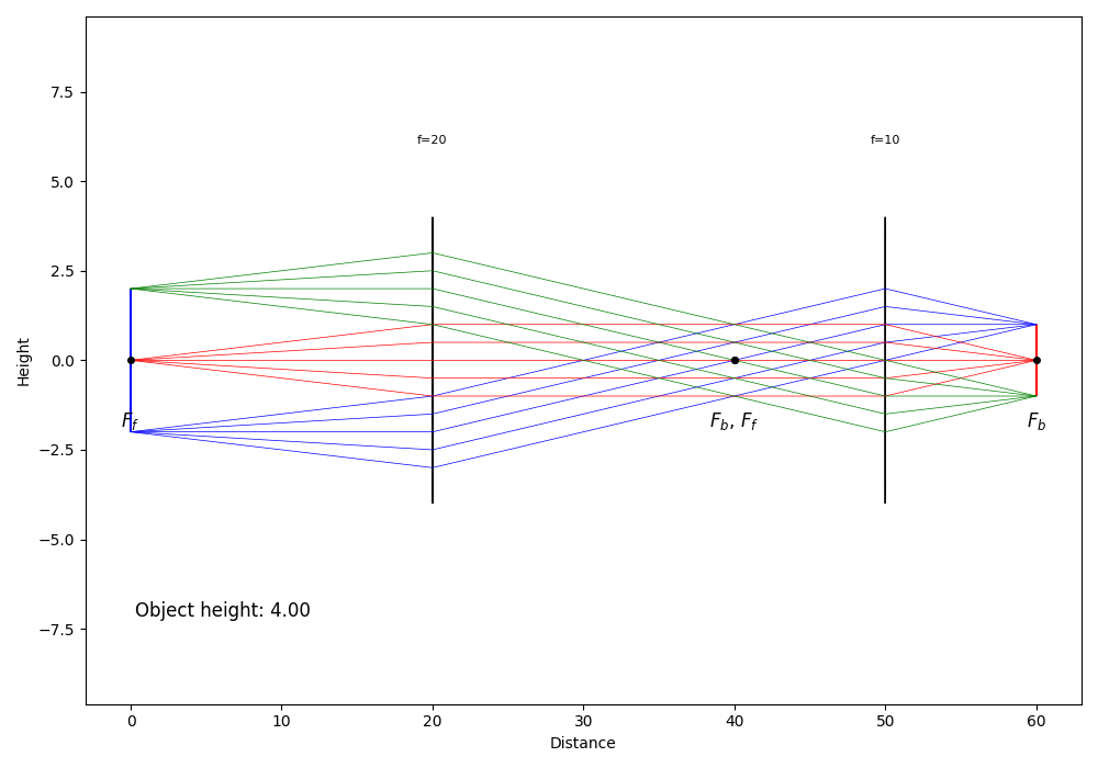
>>> from raytracing import *
>>> path = ImagingPath() # define an imaging path
>>> #set the desire properties
>>> path.objectHeight=4
>>> path.fanAngle=0.1
>>> path.fanNumber=5
>>> # use append() to add elements to the imaging path
>>> path.append(Space(d=20))
>>> path.append(Lens(f=20,label="f=20"))
>>> path.append(Space(d=30))
>>> path.append(Lens(f=10,label="f=10"))
>>> path.append(Space(d=10))
>>> #display the imeging path
>>> path.display()
And the following figure will be plotted:
-
NA()¶ This function returns the numerical aperture of the component or imaging system, which is the sin of the axial ray angle, times the index of refraction.
It is not always appreciated that the NA of an optical system is meaningful mostly in “finite conjugate” situations, that is, when either the object and the image are at small, finite distances. In practice, this means microscope objectives and 4f relays for example. On the other hand, infinite conjugate systems are better described by their f-number. A system is designed as either a finite-conjugate system or an infinite-conjugate: this is a design decision. See Smith “Modern Optical Engineering” Section 6.7 Apertures and Image Illumination.
Returns: NA Return type: float
-
apertureStop()¶ The “aperture stop” is an aperture in the system that limits the cone of angles originating from zero height at the object plane.
Returns: apertureStop – Returns an array including the position (index [0] of the output) and diameter (index [1] of the output) of the aperture stop. If there are no elements of finite diameter (i.e. all optical elements are infinite in diameters), then there is no aperture stop in the system and the size of the aperture stop is infinite (+Inf). Return type: (float,float) Examples
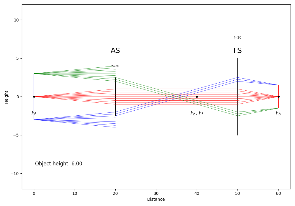
>>> from raytracing import *
>>> path = ImagingPath() # define an imaging path
>>> path.objectHeight=6
>>> # use append() to add elements to the imaging path
>>> path.append(Space(d=20))
>>> path.append(Lens(f=20,diameter=5,label="f=20"))
>>> path.append(Space(d=30))
>>> path.append(Lens(f=10,diameter=10,label="f=10"))
>>> path.append(Space(d=10))
>>> print('The position of aperture stop is:', path.apertureStop()[0])
The position of aperture stop is: 20.0
>>> print('The diameter of aperture stop is:',path.apertureStop()[1])
The diameter of aperture stop is: 5
Also, as the following, you can use display() to follow the rays in the imaging path and view the aperture stop and field stop. Since the diameter of the first lens (f=20) is limited, this is the aperture stop in the imaging path.
>>> path.display()
See also
raytracing.ImagingPath.apertureStopPosition(),raytracing.ImagingPath.apertureStopDiameter(),raytracing.ImagingPath.fieldStop()Notes
Strategy: we take a ray height and divide by real aperture diameter at that position. Some elements may have a finite length (e.g., Space() or ThickLens()), so we always calculate the ratio before propagating inside the element and after having propagated through the element. The position where the absolute value of the ratio is maximum is the aperture stop.
-
append(matrix)¶ This function adds an element at the end of the path.
Parameters: matrix (object of matrix class) – This parameter can be an element defined ABCD matrix like Lens, Space,… Returns: matrix – The new appended matrix with the input matrix at the end Return type: object of matrix class Examples
>>> from raytracing import *
>>> # define an empty matrix group
>>> matGrp=MatrixGroup()
>>> matGrp.append(Space(d=10)) # add a matrix of space (d=10)
>>> matGrp.append(Lens(f=10)) # add a matrix of a lens (f=10)
>>> matGrp.append(Space(d=10)) # add a matrix of space (d=10)
>>> print(matGrp) # print to see the output ABCD matrix
|  0.000   10.000 |
|                 |
| -0.100    0.000 |
f=10.000
-
axialRay()¶ This function returns the axial ray of the system, also known as the marginal ray for a point on axis (y=0) at the object.
Returns: axialRay – The properties (i.e. height and the angle of the marginal ray). Another axial can be obtained with the opposite of the angle. Return type: object of Ray class
-
backFocalLength()¶ The focal lengths measured from the back vertex. This is the distance between the surface and the focal point. When the principal plane is not at the surface (which is usually the case in anything except a thin lens), the back and front focal lengths will be different from effective focal lengths. The effective focal lengths is always measured from the principal planes, but the BFL and FFL are measured from the vertex.
Returns: backFocalLength – Returns the BFL Return type: float Examples
Since this function returns the BFL, if the focal distance of an object is 5 and the back vertex is 2, we expect to have back focal length of 3, as the following example:
>>> from raytracing import *
>>> # M1 is an ABCD matrix of a lens (f=5)
>>> M1= Matrix(A=1,B=0,C=-1/5,D=1,physicalLength=0,backVertex=2,label='Lens')
>>> BFL=M1.backFocalLength()
>>> print('the back focal distance:' , BFL)
the back focal distance: 3.0
See also
raytracing.Matrix.focalDistances(),raytracing.Matrix.effectiveFocalLengths(),raytracing.Matrix.frontFocalLength()Notes
If the matrix is the result of the product of several matrices, we may not know where the front and back vertices are. In that case, we return None (or undefined).
The front and back focal lengths will be different if the index of refraction is different on both sides.
-
backwardConjugate()¶ With an image at the back edge of the element, where is the object ? Distance before the element by which a ray must travel to reach the conjugate plane at the back of the element. A positive distance means the object is “distance” in front of the element (or to the left, or before).
Returns: backwardConjugate – - index [0] output object is the distance of the image in front of the element
- and index [1] is the conjugate matrix.
Return type: object Examples
>>> from raytracing import *
>>> # M1 is an ABCD matrix of an object
>>> M1= Matrix(A=2,B=1,C=5,D=3,physicalLength=2,label='Lens')
>>> Image=M1.backwardConjugate()
>>> print('The position of the image:' , Image[0])
The position of the image: -0.5
>>> print(Image[1]) #print the conjugate matrix
|  2.000    0.000 |
|                 |
|  5.000    0.500 |
f=-0.200
See also
Notes
M2 = M1*Space(distance) M2.isImaging == True
-
chiefRay(y=None)¶ This function returns the chief ray for a height y at object. The chief ray for height y is the ray that goes through the center of the aperture stop.
Parameters: y (float) – The starting height of the chief ray at the object (default=None) If no height is provided, then the function uses the limit of the field of view. Returns: chiefRay – The properties (i.e. height and the angle of the chief ray.) Return type: object of Ray class Examples
>>> from raytracing import *
>>> path = ImagingPath() # define an imaging path
>>> # use append() to add elements to the imaging path
>>> path.append(Space(d=20))
>>> path.append(Lens(f=20,diameter=2,label="f=20"))
>>> path.append(Space(d=30))
>>> path.append(Lens(f=10,diameter=10,label="f=10"))
>>> path.append(Space(d=10))
>>> print(path.chiefRay())
y =  3.333
theta = -0.167
z = 0.000
See also
raytracing.ImagingPath.marginalRays(),raytracing.ImagingPath.axialRay(),raytracing.ImagingPath.principalRay()Notes
The calculation is simple: obtain the transfer matrix to the aperture stop, then we know that the input ray (which we are looking for) will end at y=0 at the aperture stop. If the element B in the transfer matrix for the imaging path is zero, there is no value for the height and angle that makes a proper chief ray. So the function will return None. If there is no aperture stop, there is no chief ray either. None is also returned.
-
determinant¶ The determinant of the ABCD matrix is always frontIndex/backIndex, which is often 1.0. We make a calculation exception when C == 0 and B is infinity: since B is never really infinity, but C can be precisely zero (especially in free space), then B*C is zero in that particular case.
-
display(rays=None, raysList=None, removeBlocked=True, comments=None, onlyPrincipalAndAxialRays=None, limitObjectToFieldOfView=None, interactive=True, filePath=None)¶ Display the optical system and trace the rays.
Parameters: - rays (Rays instance) –
- raysList (list of Rays or list of list of Ray) –
- onlyPrincipalAndAxialRays (bool (Optional)) – If True, only the principal rays will appear on the plot (default=True)
- removeBlocked (bool (Optional)) – If True, the blocked rays are removed (default=False)
- comments (string) – If comments are included they will be displayed on a graph in the bottom half of the plot. (default=None)
-
displayHalfHeight()¶ A reasonable height for display purposes for an element, whether it is infinite or not. If the element is infinite, the half-height is currently set to ‘4’ or to the specified minimum half height. If not, it is the apertureDiameter/2. :param minSize: The minimum size to be considered as the aperture half height :type minSize: float
Returns: halfHeight – The half height of the optical element Return type: float
-
displayWithObject(diameter, fanAngle=None, fanNumber=3, rayNumber=3, removeBlocked=True, comments=None)¶ Display the optical system and trace the rays.
Parameters: - diameter (float) – Diameter of the object.
- fanAngle (float (default=None)) – the half angle for the rays. If None, it will be chosen optimally
- fanNumber (float (default=3)) – the number of rays originating from a point
- rayNumber (float (default=3)) – the number of points on the object from which rays will emerge
- removeBlocked (bool (Optional)) – If True, the blocked rays are removed (default=False)
- comments (string) – If comments are included they will be displayed on a graph in the bottom half of the plot. (default=None)
-
effectiveFocalLengths()¶ The effective focal lengths calculated from the power (C) of the matrix.
There are in general two effective focal lengths: front effective and back effective focal lengths (not to be confused with back focal and front focal lengths which are measured from the physical interface). The easiest way to calculate this is to use f = -1/C for current matrix, then flipOrientation and f = -1/C
Returns: effectiveFocalLengths – Returns the effective focal lengths in the forward and backward directions. When in air, both are equal. Return type: array See also
Examples
>>> from raytracing import *
>>> # M1 is an ABCD matrix of a lens (f=5)
>>> M1= Matrix(A=1,B=0,C=-1/5,D=1,physicalLength=0,label='Lens')
>>> f2=M1.effectiveFocalLengths()
>>> print('focal distances:' , f2)
focal distances: FocalLengths(f1=5.0, f2=5.0)
This function has the same out put as effectiveFocalLengths() >>> f1=M1.focalDistances() >>> print(‘focal distances:’ , f1) focal distances: FocalLengths(f1=5.0, f2=5.0)
-
entrancePupil()¶ The entrance pupil is the image of the aperture stop as seen from the object. To obtain this image, we simply need to know the transfer matrix to the aperture stop, then find the “backward” conjugate, which means finding the position of the “image” (the entrance pupil) that would lead to the “object” (aperture stop) at the end of the transfer matrix. All the terminology is such that it assumes the “object” is at the front and the “image” is at the back, so we need to invert the magnification.
Returns: entrancePupil – the position of the pupil relative to input reference plane (positive means to the right) and its diameter. Return type: (float,float) Examples
>>> path = ImagingPath() # define an imaging path
>>> path.objectHeight=6
>>> # use append() to add elements to the imaging path
>>> path.append(Space(d=20))
>>> path.append(Lens(f=20,diameter=5,label="f=20"))
>>> path.append(Space(d=30))
>>> path.append(Lens(f=10,diameter=10,label="f=10"))
>>> path.append(Space(d=10))
>>> print('The (position,diameter) of entrance pupil:', path.entrancePupil())
The (position,diameter) of entrance pupil: Stop(z=20.0, diameter=5.0)
-
fNumber()¶ This function returns the f-number of the component or system by dividing the diameter of the entrance pupil by the effective focal length of the system.
It is not always appreciated that the f-number of an optical system is meaningful mostly in “infinite conjugate” situations, that is, when either the object or the image is at infinity. In practice, this means with photography and telescopes for example. On the other hand, finite conjugate systems are better described by their NA. For elements, we calculate the f-number of lenses by assuming they are used with an object at infinity. A system is designed as either a finite-conjugate system or an infinite-conjugate: this is a design decision. See Smith “Modern Optical Engineering” Section 6.7 Apertures and Image Illumination.
Returns: fNumber Return type: float
-
fieldOfView()¶ The field of view is the length visible before the chief rays on either side are blocked by the field stop.
Returns: fieldOfView – length of object that can be visible at the image plane. It can be infinity if there is no field stop. Return type: float Examples
>>> from raytracing import *
>>> path = ImagingPath() # define an imaging path
>>> path.objectHeight=6
>>> # use append() to add elements to the imaging path
>>> path.append(Space(d=20))
>>> path.append(Lens(f=20,diameter=5,label="f=20"))
>>> path.append(Space(d=30))
>>> path.append(Lens(f=10,diameter=10,label="f=10"))
>>> path.append(Space(d=10))
>>> print('field of view :', path.fieldOfView())
field of view : 6.666665124862807
Notes
Strategy: take ray at various heights from object and aim at center of pupil (chief ray from that point) until ray is blocked. It is possible to have finite diameter elements but still an infinite field of view and therefore no Field stop.
-
fieldStop()¶ The field stop is the aperture that limits the image size (or field of view) It is possible to have finite diameter elements but still an infinite field of view and therefore no Field stop. In fact, if only a single element has a finite diameter, there is no field stop (only an aperture stop). The limit is arbitrarily set to maxHeight.
Returns: fieldStop – the output is the (position, diameter) of the field stop. If there are no elements of finite diameter (i.e. all optical elements are infinite in diameters), then there is no field stop and no aperture stop in the system and their sizes are infinite. Return type: (float,float) Examples
>>> from raytracing import *
>>> path = ImagingPath() # define an imaging path
>>> path.objectHeight=6
>>> # use append() to add elements to the imaging path
>>> path.append(Space(d=20))
>>> path.append(Lens(f=20,diameter=5,label="f=20"))
>>> path.append(Space(d=30))
>>> path.append(Lens(f=10,diameter=10,label="f=10"))
>>> path.append(Space(d=10))
>>> print('The position of field stop is:', path.apertureStop()[0])
The position of field stop is: 20.0
>>> print('The diameter of field stop is:',path.apertureStop()[1])
The diameter of field stop is: 5
Also, as the following, you can use display() to follow the rays in the imaging path and view the aperture stop and field stop. The second lens in the imaging path (f=10) is the field stop.
>>> path.display()
Notes
Strategy: We want to find the exact height from the object where it is blocked by an aperture (which will become the field stop). We look for the point that separates the “unblocked” ray from the “blocked” ray.
To do so, we take a ray at various heights starting at y=0 from object with a finite increment “dy” and aim at center of pupil (i.e. chief ray from that height) until ray is blocked. If it is not blocked, increase dy and increase y by dy. When it is blocked, we turn around and increase by only half the dy, then we continue until it is unblocked, turn around, divide dy by 2, etc… This rapidly converges to the position at which the ray is blocked, which is the field stop half diameter. This strategy is better than linearly going through object heights because the precision can be very high without a long calculation time.
-
flipOrientation()¶ Flip the orientation (forward-backward) of this group of elements. Each element is also flipped individually.
-
focalDistances()¶ This is the synonym of effectiveFocalLengths()
Returns: focalDistances – Returns the effective focal lengths on either side. Return type: array Examples
>>> from raytracing import *
>>> # M1 is an ABCD matrix of a lens (f=5)
>>> M1= Matrix(A=1,B=0,C=-1/5,D=1,physicalLength=0,label='Lens')
>>> f1=M1.focalDistances()
>>> print('focal distances:' , f1)
focal distances: FocalLengths(f1=5.0, f2=5.0)
This function has the same out put as effectiveFocalLengths()
>>> f2=M1.effectiveFocalLengths()
>>> print('focal distances:' , f2)
focal distances: FocalLengths(f1=5.0, f2=5.0)
-
focusPositions(z)¶ Positions of both focal points on either side of the element.
The front and back focal spots will be different if the index of refraction is different on both sides.
Parameters: z (float) – Position from where the positions are calculated Returns: focusPositions – An array of front focal position and the back focal position. Return type: array Examples
>>> from raytracing import *
>>> # M1 is an ABCD matrix of a lens (f=5)
>>> M1= Matrix(A=1,B=0,C=-1/5,D=1,physicalLength=4,frontVertex=-1,backVertex=5,label='Lens')
>>> Position0=M1.focusPositions(z=0)
>>> print('focal positions (F,B):' , Position0)
focal positions (F,B): CardinalPoint(z1=-5.0, z2=9.0)
And if we move object 2 units:
>>> Position2=M1.focusPositions(z=2)
>>> print('focal positions (F,B):' , Position2)
focal positions (F,B): CardinalPoint(z1=-3.0, z2=11.0)
-
forwardConjugate()¶ With an object at the front edge of the element, where is the image? Distance after the element by which a ray must travel to reach the conjugate plane of the front of the element. A positive distance means the image is “distance” beyond the back of the element (or to the right, or after).
Returns: forwardConjugate – - index [0] output object is the distance of the image at the back of the element
- and index [1] is the conjugate matrix.
Return type: object Examples
>>> from raytracing import *
>>> # M1 is an ABCD matrix of an object
>>> M1= Matrix(A=3,B=1,C=5,D=2,physicalLength=0,label='Lens')
>>> Image=M1.forwardConjugate()
>>> print('The position of the image:' , Image[0])
The position of the image: -0.5
>>> print(Image[1]) #print the conjugate matrix
|  0.500    0.000 |
|                 |
|  5.000    2.000 |
f=-0.200
Notes
M2 = Space(distance)*M1 M2.isImaging == True
-
forwardSurfaces¶ A list of surfaces that represents the element for drawing purposes
-
frontFocalLength()¶ The focal lengths measured from the front vertex. This is the distance between the surface and the focal point. When the principal plane is not at the surface (which is usually the case in anything except a thin lens), the back and front focal lengths will be different from effective focal lengths. The effective focal lengths is always measured from the principal planes, but the BFL and FFL are measured from the vertices.
Returns: frontFocalLength – Returns the FFL Return type: float Examples
In the following example, we have defined an object(f=5) with physical length of 4. And the front vertex is placed one unit before the front principal plane. There for the front focal length will be 4.
>>> from raytracing import *
>>> # M1 is an ABCD matrix of a lens (f=5)
>>> M1= Matrix(A=1,B=0,C=-1/5,D=1,physicalLength=4,frontVertex=-1,label='Lens')
>>> FFL=M1.frontFocalLength()
>>> print('the front focal distance:' , FFL)
the front focal distance: 4.0
See also
raytracing.Matrix.focalDistances(),raytracing.Matrix.effectiveFocalLengths(),raytracing.Matrix.backFocalLength()Notes
If the matrix is the result of the product of several matrices, we may not know where the front and back vertices are. In that case, we return None (or undefined).
The front and back focal lengths will be different if the index of refraction is different on both sides.
-
halfFieldOfView()¶ The half field of view is the maximum height visible before its chief ray is blocked by the field stop. A ray at that height is the principal ray, of “highest chief ray”.
Returns: halfFieldOfView – maximum ray height that can still be visible at the image plane. It can be infinity if there is no field stop. Return type: float Examples
>>> from raytracing import *
>>> path = ImagingPath() # define an imaging path
>>> path.objectHeight=6
>>> # use append() to add elements to the imaging path
>>> path.append(Space(d=20))
>>> path.append(Lens(f=20,diameter=5,label="f=20"))
>>> path.append(Space(d=30))
>>> path.append(Lens(f=10,diameter=10,label="f=10"))
>>> path.append(Space(d=10))
>>> print('field of view :', path.fieldOfView())
field of view : 6.666665124862807
Notes
Strategy: take ray at various heights from object and aim at center of pupil (chief ray from that point) until ray is blocked. It is possible to have finite diameter elements but still an infinite field of view and therefore no Field stop.
-
hasApertureStop()¶ Returns True if this ImagingPath has an aperture stop. The presence of a single finite diameter element is usually sufficient to have an aperture stop.
-
hasFieldStop()¶ Returns True if this ImagingPath has a field stop.
The presence of a single finite diameter element is not sufficient to have a field stop: we must have at least two finite aperture elements (maybe more depending on position) to have a field stop. If the system has no field stop, then the fieldOfView will be infinite.
-
hasFiniteApertureDiameter()¶ True if ImagingPath has at least one element of finite diameter
-
hasPower¶ If True, then there is a non-null focal length because C!=0. We compare to an epsilon value, because computational errors can occur and lead to C being very small, but not 0.
Examples
>>> from raytracing import *
>>> # M1 is an ABCD matrix of a lens (f=10)
>>> M1= Matrix(A=1,B=0,C=-1/10,D=1,physicalLength=2,label='Lens')
>>> print('hasPower:' , M1.hasPower)
hasPower: True
>>> # M2 is an ABCD matrix of free space (d=2)
>>> M2= Matrix(A=1,B=2,C=0,D=1,physicalLength=2,label='Lens')
>>> print('hasPower:' , M2.hasPower)
hasPower: False
-
imageSize(useObject=False)¶ The actual formal definition of image size is the object field of view multiplied by magnification. This value is independent from the height of the object. However, if the FOV is infinite, this may not be what the user is expecting. In this case a warning is printed and we offer the possibility to use objectHeight from the class.
Parameters: useObject (bool default False) – Whether or not we use the finite objectHeight provided in the class instead of the field of view to calculate the image size. Returns: imageSize – the size of the image Return type: float Examples
>>> from raytracing import *
>>> path = ImagingPath() # define an imaging path
>>> # use append() to add elements to the imaging path
>>> path.append(Space(d=10))
>>> path.append(Lens(f=10,diameter=10,label="f=10"))
>>> path.append(Space(d=30))
>>> path.append(Lens(f=20,diameter=15,label="f=20"))
>>> path.append(Space(d=20))
>>> print('size of the image :', path.imageSize())
size of the image : 9.999998574656525
-
insert(index: int, element: raytracing.matrix.Matrix)¶ This function is used to insert a matrix at a specific index.
Parameters: - index (int) – Index where the matrix is inserted.
- element (Matrix) – Matrix object to insert. Can be a single matrix or multiple matrices within a group.
Examples
Let’s insert a 2f system in front of another 2f system to build a 4f system
>>> from raytracing import *
>>> initialGroup = MatrixGroup([Space(10), Lens(10), Space(10)])
>>> print(f"Initial 2f is imaging? {initialGroup.isImaging}")
Initial 2f is imaging? False
>>> initialGroup.insert(0, MatrixGroup([Space(15), Lens(15), Space(15)]))
>>> print(f"Final 4f is imaging? {initialGroup.isImaging}")
Final 4f is imaging? True
Let’s insert an aperture between two 2f systems with infinite diameters >>> from raytracing import * >>> system = MatrixGroup([Space(10), Lens(10), Space(10), Space(10), Lens(10), Space(10)]) >>> print(f”Has finite diameter? {system.hasFiniteApertureDiameter()}”) Has finite diameter? False
>>> system.insert(3, Aperture(50))
>>> print(f"Has finite diameter? {system.hasFiniteApertureDiameter()}")
Has finite diameter? True
See also
-
intermediateConjugates()¶ This function calculates the position and the magnification of the conjugate planes.
Returns: planes – The list of position and magnification of conjugate planes Return type: List Examples
The first index is the position of the conjugate plane and the second index is the magnification
>>> from raytracing import *
>>> # define the elements in the optical path
>>> Lens1=Lens(f=10,label='Lens1') # lens f=10
>>> Spc1=Space(d=30,label='Space1') # space d=10
>>> Lens2=Lens(f=20,label='Lens2') # lens f=20
>>> matGrp=MatrixGroup(elements=[Lens1,Spc1,Lens2]) # make a matrix group of the created elements
>>> # print to see the transfer matrices of the space and the lens
>>> print(matGrp.intermediateConjugates())
[[90.0, -2.0]]
-
isImaging¶ If B=0, then the matrix represents that transfer from a conjugate plane to another (i.e. object at the front edge and image at the back edge).
Examples
>>> from raytracing import *
>>> # M1 is an ABCD matrix of a lens (f=10)
>>> M1= Matrix(A=1,B=0,C=-1/10,D=1,physicalLength=2,label='Lens')
>>> print('isImaging:' , M1.isImaging)
isImaging: True
>>> # M2 is an ABCD matrix of free space (d=2)
>>> M2= Matrix(A=1,B=2,C=0,D=1,physicalLength=2,label='Lens')
>>> print('isImaging:' , M2.isImaging)
isImaging: False
Notes
In this case: A = transverse magnification D = angular magnification And as usual, C = -1/f (always).
-
lagrangeInvariant()¶ The lagrange invariant is the optical invariant calculated with the principal and axial rays. It represents the maximum optical invariant for which both rays can propagate unimpeded.
Returns: lagrangeInvariant – The value of the lagrange invariant for the system Return type: float
-
largestDiameter¶ Largest finite diameter in all elements
-
load(filePath, append=False)¶ A MatrixGroup saved with save() can be loaded using this function.
Parameters: - filePath (str or PathLike or file-like object) – A path, or a Python file-like object, or possibly some backend-dependent object. Must be provided in OS-dependent format.
- append (bool) – If True, the loaded elements will be appended to the current list of elements.
-
magnification()¶ The magnification of the element
Returns: magnification – You can access via indexes or .transverse and .angular index [0] output object is A in the matrix and index [1] is D in the matrix. Return type: namedtuple (transverse, angular) Examples
>>> from raytracing import *
>>> # M1 is an ABCD matrix of an object
>>> Mat= Matrix(A=1,B=0,C=-1/5,D=1,physicalLength=0,label='Lens')
>>> M=Mat.magnification()
>>> print('(A , D): (',M[0],',',M[1],')')
(A , D): ( 1.0 , 1.0 )
See also
Notes
The magnification can be calculated having both A and D.
-
marginalRays(y=0)¶ This function calculates the marginal rays for a height y at object. The marginal rays for height y are the rays that hit the upper and lower edges of the aperture stop. There are always two marginal rays for any point on the object. They are symmetric on either side of the optic axis only when y=0, in which case they are called the axial rays (or just axial ray).
Parameters: y (float) – The starting height of the marginal rays at the object (default=0) In general, this could be any height, not just y=0. However, we usually want y=0 which is implicitly called “the axial ray (of the system)”, Returns: marginalRays – The properties (i.e. heights and the angles of the marginal rays.). If the default value is used at the input (y=0), both rays will be symmetrically oriented on either side of the optical axis. Return type: list of object of Ray class Examples
>>> from raytracing import *
>>> path = ImagingPath() # define an imaging path
>>> # use append() to add elements to the imaging path
>>> path.append(Space(d=20))
>>> path.append(Lens(f=20,diameter=2,label="f=20"))
>>> path.append(Space(d=30))
>>> path.append(Lens(f=10,diameter=10,label="f=10"))
>>> path.append(Space(d=10))
>>> print( 'the first marginal ray is:\n', path.marginalRays()[0])
the first marginal ray is:
 y =  0.000
theta =  0.050
z = 0.000
>>> print( 'the second marginal ray is:\n', path.marginalRays()[1])
the second marginal ray is:
 y =  0.000
theta = -0.050
z = 0.000
As it can be seen in the example, the marginal rays at y=0 are symmetrically oriented on either side of the optical axis.
See also
raytracing.ImagingPath.axialRay(),raytracing.ImagingPath.chiefRay(),raytracing.ImagingPath.principalRay()Notes
The calculation is simple: obtain the transfer matrix to the aperture stop, then we know that the input ray (which we are looking for) will end at y= +/-(diameter/2) at the aperture stop. We return the largest (positive) angle first, for convenience.
-
mul_beam(rightSideBeam)¶ This function calculates the multiplication of a coherent beam with complex radius of curvature q by an ABCD matrix.
Parameters: rightSideBeam (object from GaussianBeam class) – including the beam properties Returns: outputBeam – The properties of the beam at the output of the system with the defined ABCD matrix Return type: object from GaussianBeam class Examples
>>> from raytracing import *
>>> # M1 is an ABCD matrix of a lens (f=10)
>>> M1= Matrix(A=1,B=0,C=-1/10,D=1,physicalLength=5,label='Lens')
>>> # B is a Gaussian Beam
>>> B=GaussianBeam(q=complex(4.999994928425984,0.0050356572916806525),w=1,R=5,n=1)
>>> print(M1.mul_beam(B)) #print the output properties
Complex radius: (10+0.0201j)
w(z): 1.000, R(z): 10.000, z: 5.000, λ: 0.0 nm
zo: 0.020, wo: 0.002, wo position: -10.000
-
mul_matrix(rightSideMatrix: raytracing.matrix.Matrix)¶ This function is used to combine two elements into a single matrix. The multiplication of two ABCD matrices calculates the total ABCD matrix of the system. Total length of the elements is calculated (z) but apertures are lost. We compute the first and last vertices.
Parameters: rightSideMatrix (object from Matrix class) – including the ABCD matrix and other properties of an element. Returns: - A matrix with
- a (float) – Value of the index (1,1) in the ABCD matrix of the combination of the two elements.
- b (float) – Value of the index (2,1) in the ABCD matrix of the combination of the two elements.
- c (float) – Value of the index (1,2) in the ABCD matrix of the combination of the two elements.
- d (float) – Value of the index (2,2) in the ABCD matrix of the combination of the two elements.
- frontVertex (float) – First interface used for FFL
- backVertex (float) – Last interface used for BFL
- physicalLength (float) – Length of the combination of the two elements.
Examples
Consider a Lens (f=3) and a free space (d=2). The equal ABCD matrix of this system can be calculated as the following
>>> from raytracing import *
>>> # M1 is an ABCD matrix of a lens (f=3)
>>> M1= Matrix(A=1,B=0,C=-1/3,D=1,label='Lens')
>>> # M2 is an ABCD matrix of free space (d=2)
>>> M2= Matrix(A=1,B=2,C=0,D=1,label='freeSpace')
>>> print(M1.mul_matrix(M2)) #print the total ABCD matrix
|  1.000    2.000 |
|                 |
| -0.333    0.333 |
f=3.000
Notes
If there is more than two elements, the multplication can be repeated to calculate the total ABCD matrix of the system. When combining matrices, any apertures are lost.
-
mul_ray(rightSideRay)¶ This function does the multiplication of a ray by a matrix. The output shows the propagated ray through the system. New position of ray is updated by the physical length of the matrix.
Parameters: rightSideRay (object from Ray class) – including the Ray properties Returns: outputRay – New position of the input ray after passing through the element. Return type: an object from Ray class Examples
A propagation of a ray at height 10 with angle 10 can be written as the following:
>>> from raytracing import *
>>> # M1 is an ABCD matrix of a lens (f=10)
>>> M1= Matrix(A=1,B=0,C=-1/10,D=1,physicalLength=5,label='Lens')
>>> # R is a ray
>>> R= Ray(y=10,theta=10)
>>> print('The output ray of Lens M1:\n' , M1.mul_ray(R))
The output ray of Lens M1:
 y = 10.000
theta =  9.000
z = 5.000
And after a free space (d=2)
>>> # M2 is an ABCD matrix of free space (d=2)
>>> M2= Matrix(A=1,B=2,C=0,D=1,physicalLength=2,label='freeSpace')
>>> M=M1.mul_matrix(M2)
>>> print('The output ray of Lens M1 and free space M2:\n' , M.mul_ray(R))
The output ray of Lens M1 and free space M2:
 y = 30.000
theta =  7.000
z = 7.000
See also
raytracing.Matrix.mul_matrix(),raytracing.Matrix.mul_beam(),raytracing.ray()Notes
If the ray is beyond the aperture diameter it is labelled as “isBlocked = True” but the propagation can still be calculated.
-
objectHeight Get or set the object height, at the starting edge of the ImagingPath.
-
opticalInvariant(ray1, ray2, z=0)¶ The optical invariant is a quantity that is conserved for any two rays in the system. It is very general and any two rays can be used. At a given position z, it is simply n✕(θ₁y₂ - θ₂y₁), where n is the index at that z.
In an ImagingPath, it will often be calculated with the principal and axial rays, in which case the optical invariant is called the Lagrange Invariant. The Lagrange invariant is the maximal optical invariant that guarantees neither rays will be blocked.
Parameters: - ray1 (object of Ray class) – A ray at height y1 and angle theta1 (default=None)
- ray2 (object of Ray class) – A ray at height y2 and angle theta2 (default=None)
- z (float) – A distance that shows propagation length (default=0)
Returns: opticalInvariant – The value of the optical invariant constant for ray1 and ray2
Return type: float
Examples
Since there is no input for the function, the optical invariant value is calculated for chief and marginal rays.
>>> from raytracing import *
>>> path = ImagingPath() # define an imaging path
>>> # use append() to add elements to the imaging path
>>> path.append(Space(d=10))
>>> path.append(Lens(f=10,diameter=10,label="f=10"))
>>> path.append(Space(d=30))
>>> path.append(Lens(f=20,diameter=15,label="f=20"))
>>> path.append(Space(d=20))
>>> ray1, ray2 = Ray(0.5,0.05) , Ray(3,0.25)
>>> print('optical invariant :', path.opticalInvariant(ray1,ray2))
optical invariant : 0.025000000000000022
Notes
This quantity is L = n (y1 theta2 - y2 theta1)
-
pointsOfInterest(z)¶ Any points of interest for this matrix (focal points, principal planes etc…)
-
pop(index: int)¶ This function is used to remove a matrix at a specific index.
Parameters: index (int) – Index where the matrix is removed. Returns: poppedElement – The removed matrix. Return type: Matrix Examples
Let’s remove an aperture from a 4f system: >>> from raytracing import * >>> system = MatrixGroup([Space(10), Lens(10), Space(10), Space(10), Lens(10), Space(10), Aperture(100)]) >>> print(f”Has finite diameter? {system.hasFiniteApertureDiameter()}”) Has finite diameter? True
>>> aperture = system.pop(-1) # Removes the last element
>>> print(f"Has finite diameter? {system.hasFiniteApertureDiameter()}")
Has finite diameter? False
-
principalPlanePositions(z)¶ Positions of the input and output principal planes.
Parameters: z (float) – Position from where the positions are calculated Returns: principalPlanePositions – An array of front principal plane position and the back principal plane position. Return type: array Examples
>>> from raytracing import *
>>> # M1 is an ABCD matrix of a lens (f=5)
>>> M1= Matrix(A=1,B=0,C=-1/5,D=1,physicalLength=3,frontVertex=-1,backVertex=5,label='Lens')
>>> Position0=M1.principalPlanePositions(z=0)
>>> print('PP positions (F,B):' , Position0)
PP positions (F,B): PrincipalPlanes(z1=0.0, z2=3.0)
-
principalRay()¶ This function returns the principal ray, which is the chief ray for the height y at the edge of the field of view. The chief ray is the ray that goes through the center of the aperture stop.
Returns: principalRay – The properties (i.e. height and the angle of the principal ray). Return type: object of Ray class Notes
Because of round off errors, we need to double check that the ray really goes through. We lower the height until it does if it initially does not.
-
reportEfficiency(objectDiameter=None, emissionHalfAngle=None, nRays=10000)¶ The collection efficiency of the optical system is computed and a report is printed. By default, it is computed across the field of view, but a specific object diameter can be provided as welll as an emission half angle. The analysis is based on representing each ray as a linear combination of the principal and axial rays. If the coefficients are more than 1.0, the rays will be blocked. If they are both less than 1.0, they should propagated unblocked to the image unless there is vignetting.
Parameters: - objectDiameter (float) – The size of the object for the efficiency reference. Default: field of view
- nRays (int) – Number of rays simulated to calculate efficiency. Default: 10000
-
save(filePath: str)¶ A MatrixGroup can be saved using this function and loaded with load()
Parameters: filePath (str or PathLike or file-like object) – A path, or a Python file-like object, or possibly some backend-dependent object. Must be provided in OS-dependent format.
-
saveFigure(filePath, rays=None, raysList=None, removeBlocked=True, comments=None, onlyPrincipalAndAxialRays=None, limitObjectToFieldOfView=None)¶ The figure of the imaging path can be saved using this function.
Parameters: - filePath (str or PathLike or file-like object) – A path, or a Python file-like object, or possibly some backend-dependent object. If filepath is not a path or has no extension, remember to specify format to ensure that the correct backend is used.
- rays (Rays instance) –
- raysList (list of Rays or list of list of Ray) –
- onlyPrincipalAndAxialRays (bool (Optional)) – If True, only the principal rays will appear on the plot (default=True)
- removeBlocked (bool (Optional)) – If True, the blocked rays are removed (default=False)
- comments (string) – If comments are included they will be displayed on a graph in the bottom half of the plot. (default=None)
-
subPath(zStart: float, backwards=False)¶ Secondary ImagingPath defined from a desired zStart to the end of current path or to the start of current path if ‘backwards’ is True. Used internally to trace rays from different positions.
-
trace(inputRay)¶ Trace the input ray from first element until after the last element, indicating if the ray was blocked or not.
Parameters: inputRay (object of ray class) – A ray with height y and angle theta Returns: rayTrace – Returns a ray trace (i.e. [Ray()]) starting with inputRay, followed by the ray after each element. Return type: object of ray class Notes
If an element is composed of sub-elements, the ray will also be traced in several steps. If any element blocks the ray, it will be indicated.
-
traceMany(inputRays)¶ This function trace each ray from a group of rays from front edge of element to the back edge. It can be either a list of Ray(), or a Rays() object: the Rays() object is an iterator and can be used like a list.
Parameters: inputRays (list of object of Ray class) – A List of rays, each object includes two ray. The fisr is the properties of the input ray and the second is the properties of the output ray. Returns: rayTrace – List of Ray() (i,e. a raytrace), one for each input ray. Return type: object of Ray class Examples
First, a list of 10 uniformly distributed random ray is generated and then the output of the system for the rays are calculated.
>>> from raytracing import *
>>> # M is an ABCD matrix of a lens (f=10)
>>> M= Matrix(A=1,B=0,C=-1/10,D=1,physicalLength=2,label='Lens')
>>> # inputRays is a group of random rays with uniform distribution at center
>>> nRays = 10
>>> inputRays = RandomUniformRays(yMax=0, maxCount=nRays)
>>> Tr=M.traceMany(inputRays)
>>> #index[0] of the first object in the list is the first input
>>> print('The properties of the first input ray:\n', Tr[0][0])
The properties of the first input ray:
 y =  0.000
theta =  0.153
z = 0.000
>>> #index[1] of the first object in the list is the first output
>>> print('The properties of the first output ray:\n', Tr[0][1])
The properties of the first output ray:
 y =  0.000
theta =  0.153
z = 2.000
-
traceManyThrough(inputRays, progress=True)¶ This function trace each ray from a list or a Rays() distribution from front edge of element to the back edge. Input can be either a list of Ray(), or a Rays() object: the Rays() object is an iterator and can be used like a list of rays. UniformRays, LambertianRays() etc… can be used.
Parameters: - inputRays (object of Ray class) – A group of rays
- progress (bool) – if True, the progress of the raceTrough is shown (default=Trye)
Returns: outputRays – List of Ray() (i,e. a raytrace), one for each input ray.
Return type: object of Ray class
Examples
Since the input of this example is random, we should not expect to get the same results every time.
>>> from raytracing import *
>>> # M is an ABCD matrix of a lens (f=10)
>>> M= Matrix(A=1,B=0,C=-1/10,D=1,physicalLength=2,label='Lens')
>>> # inputRays is a group of random rays with uniform distribution at center
>>> nRays = 3
>>> inputRays = RandomUniformRays(yMax=5, yMin=0, maxCount=nRays)
>>> Tr=M.traceManyThrough(inputRays)
>>> print('heights of the output rays:', Tr.yValues)
heights of the output rays: [4.323870378874155, 2.794064779525441, 0.7087442942835853]
>>> print('angles of the output rays:', Tr.thetaValues)
angles of the output rays: [-1.499826089814585, 0.7506850963379516, -0.44348989046728904]
Notes
We assume that if the user will be happy to receive Rays() as an output even if they passed a list of rays as inputs.
-
traceManyThroughInParallel(inputRays, progress=True, processes=None)¶ This is an advanced technique to gain from parallel computation: it is the same as traceManyThrough(), but splits this call in several other parallel processes using the multiprocessing module, which is os-independent.
Everything hinges on a simple pool.map() command that will apply the provided function to every element of the array, but across several processors. It is trivial to implement and the benefits are simple: if you create 8 processes on 8 CPU cores, you gain a factor of approximately 8 in speed. We are not talking GPU acceleration, but still: 1 minute is shorter than 8 minutes.
Parameters: - inputRays (object of Ray class) – A group of rays
- progress (bool) – If True, the progress in percentage of the traceTrough is shown (default=True)
Returns: outputRays – List of Ray() (i,e. a raytrace), one for each input ray.
Return type: object of Ray class
Notes
One important technical issue: Pool accesses the array in multiple processes and cannot be dynamically generated (because it is not thread-safe). We explicitly generate the list before the computation, then we split the array in #processes different lists.
-
traceThrough(inputRay)¶ Contrary to trace(), this only returns the last ray. Mutiplying the ray by the transfer matrix will give the correct ray but will not consider apertures. By “tracing” a ray, we do consider all apertures in the system.
Parameters: inputRay (object of Ray class) – A ray at height y and angle theta Returns: rayTrace – The height and angle of the last ray after propagating through the system, including apertures. Return type: object of Ray class Examples
>>> from raytracing import *
>>> # M is an ABCD matrix of a lens (f=10)
>>> M= Matrix(A=1,B=0,C=-1/10,D=1,physicalLength=2,label='Lens')
>>> # R1 is a ray
>>> R1=Ray(y=5,theta=20)
>>> Tr=M.traceThrough(R1)
>>> print('the height of traced ray is' , Tr.y,  'and the angle is', Tr.theta)
the height of traced ray is 5.0 and the angle is 19.5
Notes
If a ray is blocked, its property isBlocked will be true, and isNotBlocked will be false.
-
transferMatrices()¶ The list of Matrix() that corresponds to the propagation through this element (or group). For a Matrix(), it simply returns a list with a single element [self]. For a MatrixGroup(), it returns the transferMatrices for each individual element and appends them to a list for this group.
Returns: transferMatrices – The transfer matrix for each element in the matrix group Return type: List of matrices Examples
>>> from raytracing import *
>>> # define the elements in the optical path
>>> Spc1=Space(d=10,label='Space1') # space d=10
>>> Lens1=Lens(f=10,label='Lens1') # lens f=10
>>> matGrp=MatrixGroup(elements=[Spc1,Lens1]) # make a matrix group of the created elements
>>> # print to see the transfer matrices of the space and the lens
>>> print(matGrp.transferMatrices()[0])
|  1.000   10.000 |
|                 |
|  0.000    1.000 |
f = +inf (afocal)
>>> print(matGrp.transferMatrices()[1])
|  1.000    0.000 |
|                 |
| -0.100    1.000 |
f=10.000
-
transferMatrix(upTo=inf)¶ The transfer matrix between front edge and distance=upTo
Parameters: upTo (float) – The axial distance from the front edge of the first element (default=+Inf) Returns: transferMatrix – The transfer matrix from the front edge of the first element to the distance upTo Return type: object of matrix class Examples
>>> from raytracing import *
>>> # define the elements in the optical path
>>> Spc1=Space(d=10,label='Space1') # space d=10
>>> Len=Lens(f=10,label='Lens') # lens f=10
>>> Spc2=Space(d=10,label='Space2') # space d=10
>>> matGrp=MatrixGroup(elements=[Spc1,Len,Spc2]) # make a matrix group of the created elements
>>> print(matGrp.transferMatrix(upTo=15)) # print to see the transfer matrix in distance=15
|  0.500   10.000 |
|                 |
| -0.100    0.000 |
f=10.000
Notes
If “upTo” falls inside an element of finite length, then it will request from that element a “partial” transfer matrix for a fraction of the length. It is up to the Matrix() or MatrixGroup() to define such partial transfer matrix when possible. Quite simply, Space() defines a partial matrix as Space(d=upTo).
When using this transfer matrix, any information related to rays that have been blocked is lost: apertures are not part of the ray formalism. To find out if a ray has been blocked, you must use trace().
Methods
NA() |
This function returns the numerical aperture of the component or imaging system, which is the sin of the axial ray angle, times the index of refraction. |
__init__(elements[, label]) |
Initialize self. |
apertureStop() |
The “aperture stop” is an aperture in the system that limits the cone of angles originating from zero height at the object plane. |
axialRay() |
This function returns the axial ray of the system, also known as the marginal ray for a point on axis (y=0) at the object. |
chiefRay([y]) |
This function returns the chief ray for a height y at object. |
display([rays, raysList, removeBlocked, …]) |
Display the optical system and trace the rays. |
displayWithObject(diameter[, fanAngle, …]) |
Display the optical system and trace the rays. |
entrancePupil() |
The entrance pupil is the image of the aperture stop as seen from the object. |
fNumber() |
This function returns the f-number of the component or system by dividing the diameter of the entrance pupil by the effective focal length of the system. |
fieldOfView() |
The field of view is the length visible before the chief rays on either side are blocked by the field stop. |
fieldStop() |
The field stop is the aperture that limits the image size (or field of view) It is possible to have finite diameter elements but still an infinite field of view and therefore no Field stop. |
halfFieldOfView() |
The half field of view is the maximum height visible before its chief ray is blocked by the field stop. |
hasApertureStop() |
Returns True if this ImagingPath has an aperture stop. |
hasFieldStop() |
Returns True if this ImagingPath has a field stop. |
imageSize([useObject]) |
The actual formal definition of image size is the object field of view multiplied by magnification. |
lagrangeInvariant() |
The lagrange invariant is the optical invariant calculated with the principal and axial rays. |
marginalRays([y]) |
This function calculates the marginal rays for a height y at object. |
principalRay() |
This function returns the principal ray, which is the chief ray for the height y at the edge of the field of view. |
reportEfficiency([objectDiameter, …]) |
The collection efficiency of the optical system is computed and a report is printed. |
saveFigure(filePath[, rays, raysList, …]) |
The figure of the imaging path can be saved using this function. |
subPath(zStart[, backwards]) |
Secondary ImagingPath defined from a desired zStart to the end of current path or to the start of current path if ‘backwards’ is True. |
Inherited Methods
append(matrix) |
This function adds an element at the end of the path. |
backFocalLength() |
The focal lengths measured from the back vertex. |
backwardConjugate() |
With an image at the back edge of the element, where is the object ? Distance before the element by which a ray must travel to reach the conjugate plane at the back of the element. |
displayHalfHeight() |
A reasonable height for display purposes for an element, whether it is infinite or not. |
effectiveFocalLengths() |
The effective focal lengths calculated from the power (C) of the matrix. |
flipOrientation() |
Flip the orientation (forward-backward) of this group of elements. |
focalDistances() |
This is the synonym of effectiveFocalLengths() |
focusPositions(z) |
Positions of both focal points on either side of the element. |
forwardConjugate() |
With an object at the front edge of the element, where is the image? Distance after the element by which a ray must travel to reach the conjugate plane of the front of the element. |
frontFocalLength() |
The focal lengths measured from the front vertex. |
hasFiniteApertureDiameter() |
True if ImagingPath has at least one element of finite diameter |
insert(index, element) |
This function is used to insert a matrix at a specific index. |
intermediateConjugates() |
This function calculates the position and the magnification of the conjugate planes. |
load(filePath[, append]) |
A MatrixGroup saved with save() can be loaded using this function. |
magnification() |
The magnification of the element |
mul_beam(rightSideBeam) |
This function calculates the multiplication of a coherent beam with complex radius of curvature q by an ABCD matrix. |
mul_matrix(rightSideMatrix) |
This function is used to combine two elements into a single matrix. |
mul_ray(rightSideRay) |
This function does the multiplication of a ray by a matrix. |
opticalInvariant(ray1, ray2[, z]) |
The optical invariant is a quantity that is conserved for any two rays in the system. |
pointsOfInterest(z) |
Any points of interest for this matrix (focal points, principal planes etc…) |
pop(index) |
This function is used to remove a matrix at a specific index. |
principalPlanePositions(z) |
Positions of the input and output principal planes. |
profileFromRayTraces(rayTraces[, z]) |
|
save(filePath) |
A MatrixGroup can be saved using this function and loaded with load() |
trace(inputRay) |
Trace the input ray from first element until after the last element, indicating if the ray was blocked or not. |
traceMany(inputRays) |
This function trace each ray from a group of rays from front edge of element to the back edge. |
traceManyThrough(inputRays[, progress]) |
This function trace each ray from a list or a Rays() distribution from front edge of element to the back edge. |
traceManyThroughInParallel(inputRays[, …]) |
This is an advanced technique to gain from parallel computation: it is the same as traceManyThrough(), but splits this call in several other parallel processes using the multiprocessing module, which is os-independent. |
traceThrough(inputRay) |
Contrary to trace(), this only returns the last ray. |
transferMatrices() |
The list of Matrix() that corresponds to the propagation through this element (or group). |
transferMatrix([upTo]) |
The transfer matrix between front edge and distance=upTo |
Attributes
determinant |
The determinant of the ABCD matrix is always frontIndex/backIndex, which is often 1.0. |
fanAngle |
|
fanNumber |
|
forwardSurfaces |
A list of surfaces that represents the element for drawing purposes |
hasPower |
If True, then there is a non-null focal length because C!=0. |
isIdentity |
|
isImaging |
If B=0, then the matrix represents that transfer from a conjugate plane to another (i.e. |
largestDiameter |
Largest finite diameter in all elements |
objectHeight |
Get or set the object height, at the starting edge of the ImagingPath. |
rayNumber |
|
surfaces |