ImagingPath

class raytracing.ImagingPath(elements: list = None, label='')

Bases: MatrixGroup

ImagingPath: the main class of the module, allowing the combination of Matrix() or MatrixGroup() to be used as an imaging group with an object at the beginning.

Usage is to create the ImagingPath(), then append() elements and display(). You may change objectHeight, fanAngle, fanNumber and rayNumber.

Parameters:

elements ((Matrix)) – definitiion (default=None).
label (string) – The label for the imaging path

objectHeight

The full height of object can be defined using this attribute (default=10.0)

Type:: float

objectPosition

This attribute defines the position of the object which must be defined zero for now. (default=0)

Type:: float

fanAngle

This value indicates full fan angle in radians for rays (default=0.1)

Type:: float

fanNumber

This value indicates the number of fans from the object (default=3)

Type:: int

precision

The accuracy to be considered when calculating the field stop (default=0.001)

Type:: float

maxHeight

The maximum height to be considered when calculating the field stop (default=10000.0)

Type:: float

showObject

If True, the object will be shown on display (default=True)

Type:: bool

showImages

If True, the image will be shown on display (default=True)

Type:: bool

showEntrancePupil

If True, the entrance pupil will be shown on display (default=False)

Type:: bool

showElementLabels

If True, the labels of the elements will be shown on display (default=True)

Type:: bool

showPointsOfInterest

If True, the points of interests will be shown on display (default=True)

Type:: bool

showPointsOfInterestLabels

If True, the labels of the points of interests will be shown on display (default=True)

Type:: bool

Examples

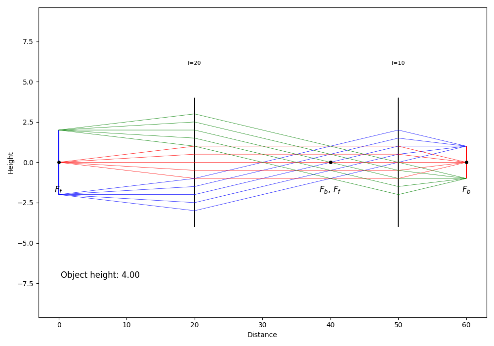
>>> from raytracing import *
>>> path = ImagingPath() # define an imaging path
>>> #set the desire properties
>>> path.objectHeight=4
>>> path.fanAngle=0.1
>>> path.fanNumber=5
>>> # use append() to add elements to the imaging path
>>> path.append(Space(d=20))
>>> path.append(Lens(f=20,label="f=20"))
>>> path.append(Space(d=30))
>>> path.append(Lens(f=10,label="f=10"))
>>> path.append(Space(d=10))
>>> #display the imeging path
>>> path.display()

And the following figure will be plotted:

NA()

This function returns the numerical aperture of the component or imaging system, which is the sin of the axial ray angle, times the index of refraction.

It is not always appreciated that the NA of an optical system is meaningful mostly in “finite conjugate” situations, that is, when either the object and the image are at small, finite distances. In practice, this means microscope objectives and 4f relays for example. On the other hand, infinite conjugate systems are better described by their f-number. A system is designed as either a finite-conjugate system or an infinite-conjugate: this is a design decision. See Smith “Modern Optical Engineering” Section 6.7 Apertures and Image Illumination.

Returns:: NA
Return type:: float

apertureStop()

The “aperture stop” is an aperture in the system that limits the cone of angles originating from zero height at the object plane.

Returns:: apertureStop – Returns an array including the position (index [0] of the output) and diameter (index [1] of the output) of the aperture stop. If there are no elements of finite diameter (i.e. all optical elements are infinite in diameters), then there is no aperture stop in the system and the size of the aperture stop is infinite (+Inf).
Return type:: (float,float)

Examples

>>> from raytracing import *
>>> path = ImagingPath() # define an imaging path
>>> path.objectHeight=6
>>> # use append() to add elements to the imaging path
>>> path.append(Space(d=20))
>>> path.append(Lens(f=20,diameter=5,label="f=20"))
>>> path.append(Space(d=30))
>>> path.append(Lens(f=10,diameter=10,label="f=10"))
>>> path.append(Space(d=10))
>>> print('The position of aperture stop is:', path.apertureStop()[0])
The position of aperture stop is: 20.0

>>> print('The diameter of aperture stop is:',path.apertureStop()[1])
The diameter of aperture stop is: 5

Also, as the following, you can use display() to follow the rays in the imaging path and view the aperture stop and field stop. Since the diameter of the first lens (f=20) is limited, this is the aperture stop in the imaging path.

>>> path.display()

See also

raytracing.ImagingPath.apertureStopPosition, raytracing.ImagingPath.apertureStopDiameter, raytracing.ImagingPath.fieldStop

Notes

Strategy: we take a ray height and divide by real aperture diameter at that position. Some elements may have a finite length (e.g., Space() or ThickLens()), so we always calculate the ratio before propagating inside the element and after having propagated through the element. The position where the absolute value of the ratio is maximum is the aperture stop.

axialRay()

This function returns the axial ray of the system, also known as the marginal ray for a point on axis (y=0) at the object.

Returns:: axialRay – The properties (i.e. height and the angle of the marginal ray). Another axial can be obtained with the opposite of the angle.
Return type:: object of Ray class

chiefRay(y=None)

This function returns the chief ray for a height y at object. The chief ray for height y is the ray that goes through the center of the aperture stop.

Parameters:: y (float) – The starting height of the chief ray at the object (default=None) If no height is provided, then the function uses the limit of the field of view.
Returns:: chiefRay – The properties (i.e. height and the angle of the chief ray.)
Return type:: object of Ray class

Examples

>>> from raytracing import *
>>> path = ImagingPath() # define an imaging path
>>> # use append() to add elements to the imaging path
>>> path.append(Space(d=20))
>>> path.append(Lens(f=20,diameter=2,label="f=20"))
>>> path.append(Space(d=30))
>>> path.append(Lens(f=10,diameter=10,label="f=10"))
>>> path.append(Space(d=10))
>>> print(path.chiefRay())
y =  3.333
theta = -0.167
z = 0.000

Notes

The calculation is simple: obtain the transfer matrix to the aperture stop, then we know that the input ray (which we are looking for) will end at y=0 at the aperture stop. If the element B in the transfer matrix for the imaging path is zero, there is no value for the height and angle that makes a proper chief ray. So the function will return None. If there is no aperture stop, there is no chief ray either. None is also returned.

display(rays=None, raysList=None, removeBlocked=True, comments=None, onlyPrincipalAndAxialRays=None, limitObjectToFieldOfView=None, interactive=True, filePath=None)

Display the optical system and trace the rays.

Parameters:

rays (Rays instance)
raysList (list of Rays or list of list of Ray)
onlyPrincipalAndAxialRays (bool (Optional)) – If True, only the principal rays will appear on the plot (default=True)
removeBlocked (bool (Optional)) – If True, the blocked rays are removed (default=False)
comments (string) – If comments are included they will be displayed on a graph in the bottom half of the plot. (default=None)

displayWithObject(diameter, fanAngle=None, fanNumber=3, rayNumber=3, removeBlocked=True, comments=None)

Display the optical system and trace the rays.

Parameters:

diameter (float) – Diameter of the object.
fanAngle (float (default=None)) – the half angle for the rays. If None, it will be chosen optimally
fanNumber (float (default=3)) – the number of rays originating from a point
rayNumber (float (default=3)) – the number of points on the object from which rays will emerge
removeBlocked (bool (Optional)) – If True, the blocked rays are removed (default=False)
comments (string) – If comments are included they will be displayed on a graph in the bottom half of the plot. (default=None)

entrancePupil()

The entrance pupil is the image of the aperture stop as seen from the object. To obtain this image, we simply need to know the transfer matrix to the aperture stop, then find the “backward” conjugate, which means finding the position of the “image” (the entrance pupil) that would lead to the “object” (aperture stop) at the end of the transfer matrix. All the terminology is such that it assumes the “object” is at the front and the “image” is at the back, so we need to invert the magnification.

Returns:: entrancePupil – the position of the pupil relative to input reference plane (positive means to the right) and its diameter.
Return type:: (float,float)

Examples

>>> path = ImagingPath() # define an imaging path
>>> path.objectHeight=6
>>> # use append() to add elements to the imaging path
>>> path.append(Space(d=20))
>>> path.append(Lens(f=20,diameter=5,label="f=20"))
>>> path.append(Space(d=30))
>>> path.append(Lens(f=10,diameter=10,label="f=10"))
>>> path.append(Space(d=10))
>>> print('The (position,diameter) of entrance pupil:', path.entrancePupil())
The (position,diameter) of entrance pupil: Stop(z=20.0, diameter=5.0)

fNumber()

This function returns the f-number of the component or system by dividing the diameter of the entrance pupil by the effective focal length of the system.

It is not always appreciated that the f-number of an optical system is meaningful mostly in “infinite conjugate” situations, that is, when either the object or the image is at infinity. In practice, this means with photography and telescopes for example. On the other hand, finite conjugate systems are better described by their NA. For elements, we calculate the f-number of lenses by assuming they are used with an object at infinity. A system is designed as either a finite-conjugate system or an infinite-conjugate: this is a design decision. See Smith “Modern Optical Engineering” Section 6.7 Apertures and Image Illumination.

Returns:: fNumber
Return type:: float

fieldOfView()

The field of view is the length visible before the chief rays on either side are blocked by the field stop.

Returns:: fieldOfView – length of object that can be visible at the image plane. It can be infinity if there is no field stop.
Return type:: float

Examples

>>> from raytracing import *
>>> path = ImagingPath() # define an imaging path
>>> path.objectHeight=6
>>> # use append() to add elements to the imaging path
>>> path.append(Space(d=20))
>>> path.append(Lens(f=20,diameter=5,label="f=20"))
>>> path.append(Space(d=30))
>>> path.append(Lens(f=10,diameter=10,label="f=10"))
>>> path.append(Space(d=10))
>>> print('field of view :', path.fieldOfView())
field of view : 6.666665124862807

Notes

Strategy: take ray at various heights from object and aim at center of pupil (chief ray from that point) until ray is blocked. It is possible to have finite diameter elements but still an infinite field of view and therefore no Field stop.

fieldStop()

The field stop is the aperture that limits the image size (or field of view) It is possible to have finite diameter elements but still an infinite field of view and therefore no Field stop. In fact, if only a single element has a finite diameter, there is no field stop (only an aperture stop). The limit is arbitrarily set to maxHeight.

Returns:: fieldStop – the output is the (position, diameter) of the field stop. If there are no elements of finite diameter (i.e. all optical elements are infinite in diameters), then there is no field stop and no aperture stop in the system and their sizes are infinite.
Return type:: (float,float)

Examples

>>> from raytracing import *
>>> path = ImagingPath() # define an imaging path
>>> path.objectHeight=6
>>> # use append() to add elements to the imaging path
>>> path.append(Space(d=20))
>>> path.append(Lens(f=20,diameter=5,label="f=20"))
>>> path.append(Space(d=30))
>>> path.append(Lens(f=10,diameter=10,label="f=10"))
>>> path.append(Space(d=10))
>>> print('The position of field stop is:', path.apertureStop()[0])
The position of field stop is: 20.0

>>> print('The diameter of field stop is:',path.apertureStop()[1])
The diameter of field stop is: 5

Also, as the following, you can use display() to follow the rays in the imaging path and view the aperture stop and field stop. The second lens in the imaging path (f=10) is the field stop.

>>> path.display()

Notes

Strategy: We want to find the exact height from the object where it is blocked by an aperture (which will become the field stop). We look for the point that separates the “unblocked” ray from the “blocked” ray.

To do so, we take a ray at various heights starting at y=0 from object with a finite increment “dy” and aim at center of pupil (i.e. chief ray from that height) until ray is blocked. If it is not blocked, increase dy and increase y by dy. When it is blocked, we turn around and increase by only half the dy, then we continue until it is unblocked, turn around, divide dy by 2, etc… This rapidly converges to the position at which the ray is blocked, which is the field stop half diameter. This strategy is better than linearly going through object heights because the precision can be very high without a long calculation time.

halfFieldOfView()

The half field of view is the maximum height visible before its chief ray is blocked by the field stop. A ray at that height is the principal ray, of “highest chief ray”.

Returns:: halfFieldOfView – maximum ray height that can still be visible at the image plane. It can be infinity if there is no field stop.
Return type:: float

Examples

>>> from raytracing import *
>>> path = ImagingPath() # define an imaging path
>>> path.objectHeight=6
>>> # use append() to add elements to the imaging path
>>> path.append(Space(d=20))
>>> path.append(Lens(f=20,diameter=5,label="f=20"))
>>> path.append(Space(d=30))
>>> path.append(Lens(f=10,diameter=10,label="f=10"))
>>> path.append(Space(d=10))
>>> print('field of view :', path.fieldOfView())
field of view : 6.666665124862807

Notes

Strategy: take ray at various heights from object and aim at center of pupil (chief ray from that point) until ray is blocked. It is possible to have finite diameter elements but still an infinite field of view and therefore no Field stop.

hasApertureStop(): Returns True if this ImagingPath has an aperture stop. The presence of a single finite diameter element is usually sufficient to have an aperture stop.

hasFieldStop()

Returns True if this ImagingPath has a field stop.

The presence of a single finite diameter element is not sufficient to have a field stop: we must have at least two finite aperture elements (maybe more depending on position) to have a field stop. If the system has no field stop, then the fieldOfView will be infinite.

imageSize(useObject=False)

The actual formal definition of image size is the object field of view multiplied by magnification. This value is independent from the height of the object. However, if the FOV is infinite, this may not be what the user is expecting. In this case a warning is printed and we offer the possibility to use objectHeight from the class.

Parameters:: useObject (bool default False) – Whether or not we use the finite objectHeight provided in the class instead of the field of view to calculate the image size.
Returns:: imageSize – the size of the image
Return type:: float

Examples

>>> from raytracing import *
>>> path = ImagingPath() # define an imaging path
>>> # use append() to add elements to the imaging path
>>> path.append(Space(d=10))
>>> path.append(Lens(f=10,diameter=10,label="f=10"))
>>> path.append(Space(d=30))
>>> path.append(Lens(f=20,diameter=15,label="f=20"))
>>> path.append(Space(d=20))
>>> print('size of the image :', path.imageSize())
size of the image : 9.999998574656525

lagrangeInvariant()

The lagrange invariant is the optical invariant calculated with the principal and axial rays. It represents the maximum optical invariant for which both rays can propagate unimpeded.

Returns:: lagrangeInvariant – The value of the lagrange invariant for the system
Return type:: float

marginalRays(y=0)

This function calculates the marginal rays for a height y at object. The marginal rays for height y are the rays that hit the upper and lower edges of the aperture stop. There are always two marginal rays for any point on the object. They are symmetric on either side of the optic axis only when y=0, in which case they are called the axial rays (or just axial ray).

Parameters:: y (float) – The starting height of the marginal rays at the object (default=0) In general, this could be any height, not just y=0. However, we usually want y=0 which is implicitly called “the axial ray (of the system)”,
Returns:: marginalRays – The properties (i.e. heights and the angles of the marginal rays.). If the default value is used at the input (y=0), both rays will be symmetrically oriented on either side of the optical axis.
Return type:: list of object of Ray class

Examples

>>> from raytracing import *
>>> path = ImagingPath() # define an imaging path
>>> # use append() to add elements to the imaging path
>>> path.append(Space(d=20))
>>> path.append(Lens(f=20,diameter=2,label="f=20"))
>>> path.append(Space(d=30))
>>> path.append(Lens(f=10,diameter=10,label="f=10"))
>>> path.append(Space(d=10))
>>> print( 'the first marginal ray is:\n', path.marginalRays()[0])
the first marginal ray is:
 y =  0.000
theta =  0.050
z = 0.000
>>> print( 'the second marginal ray is:\n', path.marginalRays()[1])
the second marginal ray is:
 y =  0.000
theta = -0.050
z = 0.000

As it can be seen in the example, the marginal rays at y=0 are symmetrically oriented on either side of the optical axis.

Notes

The calculation is simple: obtain the transfer matrix to the aperture stop, then we know that the input ray (which we are looking for) will end at y= +/-(diameter/2) at the aperture stop. We return the largest (positive) angle first, for convenience.

property objectHeight: Get or set the object height, at the starting edge of the ImagingPath.

principalRay()

This function returns the principal ray, which is the chief ray for the height y at the edge of the field of view. The chief ray is the ray that goes through the center of the aperture stop.

Returns:: principalRay – The properties (i.e. height and the angle of the principal ray).
Return type:: object of Ray class

Notes

Because of round off errors, we need to double check that the ray really goes through. We lower the height until it does if it initially does not.

reportEfficiency(objectDiameter=None, emissionHalfAngle=None, nRays=10000)

The collection efficiency of the optical system is computed and a report is printed. By default, it is computed across the field of view, but a specific object diameter can be provided as welll as an emission half angle. The analysis is based on representing each ray as a linear combination of the principal and axial rays. If the coefficients are more than 1.0, the rays will be blocked. If they are both less than 1.0, they should propagated unblocked to the image unless there is vignetting.

Parameters:

objectDiameter (float) – The size of the object for the efficiency reference. Default: field of view
nRays (int) – Number of rays simulated to calculate efficiency. Default: 10000

saveFigure(filePath, rays=None, raysList=None, removeBlocked=True, comments=None, onlyPrincipalAndAxialRays=None, limitObjectToFieldOfView=None)

The figure of the imaging path can be saved using this function.

Parameters:

filePath (str or PathLike or file-like object) – A path, or a Python file-like object, or possibly some backend-dependent object. If filepath is not a path or has no extension, remember to specify format to ensure that the correct backend is used.
rays (Rays instance)
raysList (list of Rays or list of list of Ray)
onlyPrincipalAndAxialRays (bool (Optional)) – If True, only the principal rays will appear on the plot (default=True)
removeBlocked (bool (Optional)) – If True, the blocked rays are removed (default=False)
comments (string) – If comments are included they will be displayed on a graph in the bottom half of the plot. (default=None)

subPath(zStart: float, backwards=False): Secondary ImagingPath defined from a desired zStart to the end of current path or to the start of current path if ‘backwards’ is True. Used internally to trace rays from different positions.

Methods

`NA`()	This function returns the numerical aperture of the component or imaging system, which is the sin of the axial ray angle, times the index of refraction.
`__init__`([elements, label])
`apertureStop`()	The "aperture stop" is an aperture in the system that limits the cone of angles originating from zero height at the object plane.
`axialRay`()	This function returns the axial ray of the system, also known as the marginal ray for a point on axis (y=0) at the object.
`chiefRay`([y])	This function returns the chief ray for a height y at object.
`display`([rays, raysList, removeBlocked, ...])	Display the optical system and trace the rays.
`displayWithObject`(diameter[, fanAngle, ...])	Display the optical system and trace the rays.
`entrancePupil`()	The entrance pupil is the image of the aperture stop as seen from the object.
`fNumber`()	This function returns the f-number of the component or system by dividing the diameter of the entrance pupil by the effective focal length of the system.
`fieldOfView`()	The field of view is the length visible before the chief rays on either side are blocked by the field stop.
`fieldStop`()	The field stop is the aperture that limits the image size (or field of view) It is possible to have finite diameter elements but still an infinite field of view and therefore no Field stop.
`halfFieldOfView`()	The half field of view is the maximum height visible before its chief ray is blocked by the field stop.
`hasApertureStop`()	Returns True if this ImagingPath has an aperture stop.
`hasFieldStop`()	Returns True if this ImagingPath has a field stop.
`imageSize`([useObject])	The actual formal definition of image size is the object field of view multiplied by magnification.
`lagrangeInvariant`()	The lagrange invariant is the optical invariant calculated with the principal and axial rays.
`marginalRays`([y])	This function calculates the marginal rays for a height y at object.
`principalRay`()	This function returns the principal ray, which is the chief ray for the height y at the edge of the field of view.
`reportEfficiency`([objectDiameter, ...])	The collection efficiency of the optical system is computed and a report is printed.
`saveFigure`(filePath[, rays, raysList, ...])	The figure of the imaging path can be saved using this function.
`subPath`(zStart[, backwards])	Secondary ImagingPath defined from a desired zStart to the end of current path or to the start of current path if 'backwards' is True.

Inherited Methods

`append`(matrix)	This function adds an element at the end of the path.
`backFocalLength`()	The focal lengths measured from the back vertex.
`backwardConjugate`()	With an image at the back edge of the element, where is the object ? Distance before the element by which a ray must travel to reach the conjugate plane at the back of the element.
`displayHalfHeight`()	A reasonable height for display purposes for an element, whether it is infinite or not.
`effectiveFocalLengths`()	The effective focal lengths calculated from the power (C) of the matrix.
`flipOrientation`()	Flip the orientation (forward-backward) of this group of elements.
`focalDistances`()	This is the synonym of effectiveFocalLengths()
`focusPositions`(z)	Positions of both focal points on either side of the element.
`forwardConjugate`()	With an object at the front edge of the element, where is the image? Distance after the element by which a ray must travel to reach the conjugate plane of the front of the element.
`fromFocusToFocus`()	A simple method to obtain a MatrixGroup that includes all three matrices to travel from the front focus, through the lens, and then to the back focus.
`fromStruct`(theStruct)
`frontFocalLength`()	The focal lengths measured from the front vertex.
`hasFiniteApertureDiameter`()	True if ImagingPath has at least one element of finite diameter
`insert`(index, element)	This function is used to insert a matrix at a specific index.
`intermediateConjugates`()	This function calculates the position and the magnification of the conjugate planes.
`load`(filePath[, append])	A MatrixGroup saved with save() can be loaded using this function.
`magnification`()	The magnification of the element
`mul_beam`(rightSideBeam)	This function calculates the multiplication of a coherent beam with complex radius of curvature q by an ABCD matrix.
`mul_matrix`(rightSideMatrix)	This function is used to combine two elements into a single matrix.
`mul_ray`(rightSideRay)	This function does the multiplication of a ray by a matrix.
`opticalInvariant`(ray1, ray2[, z])	The optical invariant is a quantity that is conserved for any two rays in the system.
`pointsOfInterest`(z)	Any points of interest for this matrix (focal points, principal planes etc...)
`pop`(index)	This function is used to remove a matrix at a specific index.
`principalPlanePositions`(z)	Positions of the input and output principal planes.
`profileFromRayTraces`(rayTraces[, z])
`save`(filePath)	A MatrixGroup can be saved using this function and loaded with load()
`toStruct`()
`trace`(inputRay)	Trace the input ray from first element until after the last element, indicating if the ray was blocked or not.
`traceMany`(inputRays[, useOpenCL])	This function trace each ray from a group of rays from front edge of element to the back edge.
`traceManyNative`(inputRays)	This function trace each ray from a group of rays from front edge of element to the back edge.
`traceManyOpenCL`(inputRays)	This function trace each ray from a group of rays from front edge of element to the back edge.
`traceManyThrough`(inputRays[, progress, ...])	This function trace each ray from a list or a Rays() distribution from front edge of element to the back edge.
`traceManyThroughInParallel`(inputRays[, ...])	This is an advanced technique to gain from parallel computation: it is the same as traceManyThrough(), but splits this call in several other parallel processes using the multiprocessing module, which is os-independent.
`traceThrough`(inputRay)	Contrary to trace(), this only returns the last ray.
`transferMatrices`()	The list of Matrix() that corresponds to the propagation through this element (or group).
`transferMatrix`([upTo])	The transfer matrix between front edge and distance=upTo

Attributes

`Struct`
`determinant`	The determinant of the ABCD matrix is always frontIndex/backIndex, which is often 1.0.
`fanAngle`
`fanNumber`
`forwardSurfaces`	A list of surfaces that represents the element for drawing purposes
`hasPower`	If True, then there is a non-null focal length because C!=0.
`isIdentity`
`isImaging`	If B=0, then the matrix represents that transfer from a conjugate plane to another (i.e. object at the front edge and image at the back edge).
`largestDiameter`	Largest finite diameter in all elements
`objectHeight`	Get or set the object height, at the starting edge of the ImagingPath.
`rayNumber`
`surfaces`